Neural Networks in Trading: A Spatio-Temporal State Space Model for Financial Data Analysis (STSSM Block)
 80
 0

Introduction
The E-STMFlow framework is a rare example of an approach that promises efficiency and fits seamlessly into the logic of real financial markets. In the previous article, we explored the approaches proposed by the framework’s authors and got a sense of the architecture’s character — its emphasis on compactness, precision, and respect for the structure of the data being analyzed. And now, before continuing with the practical implementation, it is helpful to review the big picture once again. This helps not only to refresh your memory, but also to immerse yourself once again in the logic behind the authors' approach.
The authors have created an architecture that handles event streams very naturally. The data here is irregular and chaotic. This is very similar to how the market behaves. The price on the chart does not move in a straight line. Trading volume comes in bursts, and ticks arrive at varying rates. To extract meaning from such streams, events are first converted into a structured tensor — a three-dimensional grid that records the coordinates and time of each change. Think of it as a structured tick tape, where every movement and every pause matters. This is how the authors prepare the data stream so that the model can process it without losing any information.
The resulting tensor is passed to the Spatio-Temporal Encoder — the key module of the architecture. It transforms the stream of events into a set of features that form a picture of the motion. The Encoder detects local fluctuations and relates them to the overall dynamics. The model responds to the stream rhythm rather than to individual values. For tasks where the speed of response to changes is important, this approach offers a significant advantage.
At the heart of the encoder is the Spatio-Temporal State Space Model (STSSM). This module processes a volume of events in layers, preserving spatial patterns and taking into account their chronological sequence. As a result, the model perceives the stream as a whole: it understands impulses, pauses, and their combinations. In the context of financial markets, this is akin to the ability to detect the onset of a trend reversal or rising volatility before traditional indicators pick up on it. STSSM generates a robust representation of the data, enabling the model to distinguish between significant events and ordinary noise.
Subsequent levels of the architecture transform these features into a concrete result. In the authors' study, this result is a dense optical flow map, but the principle is universal. The model carefully prepares the signal without burdening the system with unnecessary computations. Even at the encoder level, it's clear why the solution works effectively. It is compact, cohesive, and does not complicate natural processes. In financial markets, this means being able to process a stream of ticks quickly and without delay, capturing every significant market impulse.
The authors emphasize resource efficiency. Their approach is faster than many traditional architectures, including transformers and convolutional models with a large number of layers. By properly handling the stream of events, the model obtains the maximum amount of information at minimal cost. The encoder acts as a filter, removing unnecessary data and generating signals that provide a real advantage in data stream processing.
Another important point is maintaining temporal consistency. The event stream may be erratic, with sudden spikes and long pauses. The encoder creates a sequential representation that reflects the internal stream rhythm without sacrificing local precision. In financial markets, this is equivalent to a trader recognizing that a sharp market impulse may be lurking behind a period of calm and reacting to it in a timely manner.
Importantly, the authors' approach remains simple in essence. Everything is based on precise event discretization, STSSM processing, and compact convolutions. This solution demonstrates that powerful analytics are possible without unnecessary complexity, and that is precisely what makes E-STMFlow appealing for practical applications.
The authors' visualization of the E-STMFlow framework is shown below.

In the previous article, we decided to apply the approaches proposed by the framework's authors to the field of spiking solutions. This is entirely consistent with the logic of event-driven models. Furthermore, we have implemented an embedding stack that neatly prepares the event stream, creating a convenient structure for further analysis. It acts as a filter, allowing the model to recognize rhythm and patterns.
Today we're taking the next step and beginning to implement the heart of the encoder — the STSSM block. It is this module that will link local events to the global dynamics of the stream, creating a stable representation of the data. This is particularly important for financial data streams. The market never moves in a straight line. Ticks arrive at varying rates, and volumes can change instantaneously. The STSSM block will allow the model to perceive these impulses holistically, treat pauses and bursts as part of the bigger picture, and extract key features for further analysis.
Moving on to the practical part of the work, it is important to emphasize right away that the STSSM block is not just a module, but a complex, multi-level structure comprising several interconnected components. Its architecture resembles a carefully designed machine in which each part plays its own role, and together they provide a holistic view of the event stream. To make the process clear and easy to follow, we will build the block step by step, working our way up through its hierarchy from the bottom. This approach helps you avoid getting lost in the details and ensures you have a clear understanding of how each element contributes to the final result.
Spike-SSM Module
The first step will be to implement the SSM module. This component can be compared to the foundation of a building: it provides the basis for event processing, neatly organizing the stream and capturing its internal dynamics. In a financial context, this is similar to the work of a trader who first closely monitors changes in volume and price fluctuations before drawing conclusions about the market’s direction. The SSM module performs a similar function: it detects local changes and uses them to generate structured features that will be used at subsequent levels of the block.
We have repeatedly discussed the importance of taking into account both temporal and spatial dependencies when analyzing event streams. In this work, the 2D-SSM module is used to implement this functionality; it is capable of detecting changes not only over time but also across various data dimensions. In a market analogy, this is similar to a trader who simultaneously monitors price fluctuations and trading volume, relating each movement to the overall market context. For the spiking version of the algorithm, we implement a new class, CNeuronSpike2DSSMOCL, which inherits the basic capabilities of the neural element and adapts them to work with streams of spiking events.
class CNeuronSpike2DSSMOCL  :  public CNeuronBaseOCL
  {
protected:
   uint                    iWindowOut;
   uint                    iUnitsOut;
   //---
   CNeuronBaseOCL          cHiddenStates;
   CLayer                  cProjectionX_Time;
   CLayer                  cProjectionX_Variable;
   CNeuronSpikeConvBlock   cA;
   CNeuronSpikeConvBlock   cBC_Time;
   CNeuronSpikeConvBlock   cBC_Variable;
   CNeuronBaseOCL          cB_Time;
   CNeuronBaseOCL          cB_Variable;
   CNeuronBaseOCL          cC_Time;
   CNeuronBaseOCL          cC_Variable;
   CNeuronSpikeConvBlock   cDelta_Time;
   CNeuronSpikeConvBlock   cDelta_Variable;
   //---
   virtual bool      feedForward(CNeuronBaseOCL *NeuronOCL) override;
   virtual bool      feedForwardSSM2D(void);
   //---
   virtual bool      calcInputGradients(CNeuronBaseOCL *NeuronOCL) override;
   virtual bool      calcInputGradientsSSM2D(void);
   virtual bool      updateInputWeights(CNeuronBaseOCL *NeuronOCL) override;

public:
                     CNeuronSpike2DSSMOCL(void)  {};
                    ~CNeuronSpike2DSSMOCL(void)  {};
   //---
   virtual bool      Init(uint numOutputs, uint myIndex, COpenCLMy *open_cl,
                          uint window_in, uint window_out, uint units_in, uint units_out,
                          ENUM_OPTIMIZATION optimization_type, uint batch);
   //---
   virtual int       Type(void)   const   {  return defNeuronSpike2DSSMOCL; }
   //---
   virtual bool      Save(int const file_handle);
   virtual bool      Load(int const file_handle);
   //---
   virtual bool      WeightsUpdate(CNeuronBaseOCL *source, float tau) override;
   //---
   virtual void      SetActivationFunction(ENUM_ACTIVATION value) override { };
   virtual void      SetOpenCL(COpenCLMy *obj) override;
   virtual void      TrainMode(bool flag) override;
   //---
   virtual bool      Clear(void) override;
  };
The class architecture is designed as a finely tuned system of filters and transformation stages. Hidden states capture the current dynamics of the stream, just as a trader keeps the latest market impulses in mind. Projections along the temporal and spatial axes allow us to relate local changes to the overall picture, as if we were comparing instantaneous price fluctuations with the overall trend for the day. Convolution blocks (cA, cBC_Time, cBC_Variable, and others) identify significant changes in the stream by filtering out noise, just as an experienced analyst separates random spikes in volume from a genuine market impulse.
The initialization method defines the internal architecture of the 2D-SSM module and sets all the key parameters necessary for its stable operation. If we draw an analogy with trading, this process is similar to setting up a workspace. The observation windows and the number of financial instruments to analyze are determined, indicators are activated, and resources are prepared to process the stream of ticks. Without such preparation, any model loses its sensitivity to signals and risks missing important impulses.
bool CNeuronSpike2DSSMOCL::Init(uint numOutputs, uint myIndex, COpenCLMy * open_cl,
                                uint window_in, uint window_out, uint units_in, uint units_out,
                                ENUM_OPTIMIZATION optimization_type, uint batch)
  {
   if(!CNeuronBaseOCL::Init(numOutputs, myIndex, open_cl, window_out * units_out, optimization_type, batch))
      return false;
   SetActivationFunction(None);
The algorithm begins by passing control to the parent class, where resources are allocated for the threads and the overall structure is defined. The activation function is disabled to ensure that data is transmitted without distortion.
The iWindowOut and iUnitsOut parameters specify the size of the output window and the number of elements in the sequence — this is the foundation that determines how much information will be included in each time slice. For financial data streams, this is similar to choosing a time frame and the number of candlesticks to observe in order to capture both short-term and medium-term market impulses.
   iWindowOut = window_out;
   iUnitsOut = units_out;
Next, projection blocks along the time axis (cProjectionX_Time) and the variable axis (cProjectionX_Variable) are created. For a temporal projection, the data passes through a chain consisting of a transposition, a convolution, and another transposition.
   int index = 0;
   CNeuronSpikeConvBlock *conv = NULL;
   CNeuronTransposeOCL *transp = NULL;
//--- Projection Time
   cProjectionX_Time.Clear();
   cProjectionX_Time.SetOpenCL(OpenCL);
   transp = new CNeuronTransposeOCL();
   if(!transp ||
      !transp.Init(0, index, OpenCL, units_in, window_in, optimization, iBatch) ||
      !cProjectionX_Time.Add(transp))
     {
      DeleteObj(transp);
      return false;
     }
   index++;
   conv = new CNeuronSpikeConvBlock();
   if(!conv ||
      !conv.Init(0, index, OpenCL, units_in, units_in, iUnitsOut, window_in, 1, optimization, iBatch) ||
      !cProjectionX_Time.Add(conv))
     {
      DeleteObj(conv);
      return false;
     }
   index++;
   transp = new CNeuronTransposeOCL();
   if(!transp ||
      !transp.Init(0, index, OpenCL, window_in, iUnitsOut, optimization, iBatch) ||
      !cProjectionX_Time.Add(transp))
     {
      DeleteObj(transp);
      return false;
     }
   index++;
   conv = new CNeuronSpikeConvBlock();
   if(!conv ||
      !conv.Init(0, index, OpenCL, window_in, window_in, iWindowOut, iUnitsOut, 1, optimization, iBatch) ||
      !cProjectionX_Time.Add(conv))
     {
      DeleteObj(conv);
      return false;
     }
In practice, this is similar to analyzing a tick stream. First, we change the observation perspective; then, we evaluate local impulses and trends; and finally, we map the data back to the original space to integrate it with other data streams.
A projection along the variable axis links events to various aspects of the market — volume, the rate of price change, and the strength of market impulses. So the model perceives not just movement, but its structure.
//--- Projection Variables
   cProjectionX_Variable.Clear();
   cProjectionX_Variable.SetOpenCL(OpenCL);
   index++;
   conv = new CNeuronSpikeConvBlock();
   if(!conv ||
      !conv.Init(0, index, OpenCL, window_in, window_in, iUnitsOut, units_in, 1, optimization, iBatch) ||
      !cProjectionX_Variable.Add(conv))
     {
      DeleteObj(conv);
      return false;
     }
   index++;
   transp = new CNeuronTransposeOCL();
   if(!transp ||
      !transp.Init(0, index, OpenCL, units_in, iUnitsOut, optimization, iBatch) ||
      !cProjectionX_Variable.Add(transp))
     {
      DeleteObj(transp);
      return false;
     }
   index++;
   conv = new CNeuronSpikeConvBlock();
   if(!conv ||
      !conv.Init(0, index, OpenCL, units_in, units_in, iWindowOut, iUnitsOut, 1, optimization, iBatch) ||
      !cProjectionX_Variable.Add(conv))
     {
      DeleteObj(conv);
      return false;
     }
Hidden states (cHiddenStates) and block A form the core of the analysis, carefully linking local events to the overall market picture.
//--- HiddenState
   index++;
   if(!cHiddenStates.Init(0, index, OpenCL, 2 * iUnitsOut * iWindowOut, optimization, iBatch))
      return false;
//--- A*H
   index++;
   if(!cA.Init(0, index, OpenCL, iWindowOut, iWindowOut, 2 * iWindowOut, iUnitsOut, 2, optimization, iBatch))
      return false;
It is worth noting that both components contain information for analyzing both temporal and spatial aspects. As a result, they can be processed simultaneously in parallel threads, which significantly speeds up data processing and allows the model to respond to market changes in near real time.
Block BC serves as the link between the module's core and matrices B and C. It generates these matrices simultaneously, after which they are separated into dedicated buffers for further processing.
//--- BC
   index++;
   if(!cBC_Time.Init(0, index, OpenCL, iWindowOut, iWindowOut, iUnitsOut + 1, iUnitsOut,
                                                                  1, optimization, iBatch))
      return false;
   index++;
   if(!cBC_Variable.Init(0, index, OpenCL, iWindowOut, iWindowOut, iUnitsOut + 1, iUnitsOut,
                                                                   1, optimization, iBatch))
      return false;
//--- B
   index++;
   if(!cB_Time.Init(0, index, OpenCL, iUnitsOut, optimization, iBatch))
      return false;
   cB_Time.SetActivationFunction(None);
   index++;
   if(!cB_Variable.Init(0, index, OpenCL, iUnitsOut, optimization, iBatch))
      return false;
   cB_Variable.SetActivationFunction(None);
//--- C
   index++;
   if(!cC_Time.Init(0, index, OpenCL, iUnitsOut * iUnitsOut, optimization, iBatch))
      return false;
   cC_Time.SetActivationFunction(None);
   index++;
   if(!cC_Variable.Init(0, index, OpenCL, iUnitsOut * iUnitsOut, optimization, iBatch))
      return false;
   cC_Variable.SetActivationFunction(None);
This allows signals to be integrated precisely and spatio-temporal dependencies between the various components of the stream to be captured. Matrices B and C form the basis for subsequent corrections and updates to the model's state, ensuring an accurate response to market impulses and sudden changes in volume.
Delta blocks (cDelta_Time and *cDelta_Variable) track changes in state over time and across variables, adjusting forecasts based on market dynamics. For example, a sharp spike in volume or a short-term price surge is immediately recorded and influences future forecasts, just as if an experienced trader were taking instantaneous volatility into account.
//--- Delta
   index++;
   if(!cDelta_Time.Init(0, index, OpenCL, iWindowOut, iWindowOut, iUnitsOut, iUnitsOut, 1, optimization, iBatch))
      return false;
   index++;
   if(!cDelta_Variable.Init(0, index, OpenCL, iWindowOut, iWindowOut, iUnitsOut, iUnitsOut, 1, optimization, iBatch))
      return false;
//---
   if(!Clear())
      return false;
//---
   return true;
  }
Each step of the initialization process is thoroughly checked. If an element cannot be created, the resources are released, preventing errors and crashes.
At the end, the Clear method is called, which clears all intermediate states and prepares the object to process the first data stream. In a financial market context, this is like a warm-up before a trading session — the model is ready to respond to any impulses without losing focus or structure.
As a result, the initialization method creates a complete 2D-SSM module architecture, allowing the model to view the stream of events as a single, cohesive process.
The forward pass algorithm in 2D-SSM is implemented in the feedForward method. It can be thought of as a virtual trading session. The tick stream passes through a series of analytical filters, each of which performs a specific task. First, the data enters the Projection Time chain, where each block processes events along the time axis. It is as if a trader were closely monitoring every candlestick on the chart: noting short-term fluctuations, market impulses, and sharp price movements. Each element of the projection carefully filters the signal, isolating the important parts and passing them on.
bool CNeuronSpike2DSSMOCL::feedForward(CNeuronBaseOCL * NeuronOCL)
  {
   CNeuronBaseOCL *inp = NeuronOCL;
   CNeuronBaseOCL *x_time = NULL;
   CNeuronBaseOCL *x_var = NULL;
//--- Projection Time
   int total = cProjectionX_Time.Total();
   for(int i = 0; i < total; i++)
     {
      x_time = cProjectionX_Time.At(i);
      if(!x_time ||
         !x_time.FeedForward(inp))
         return false;
      inp = x_time;
     }
The data stream is then routed to Projection Variable, where other aspects of the market are analyzed: trading volume, the rate of price change, and the strength of market impulses. Here, the model looks at the market from a different perspective — the parameter space — by linking events together. Processing these two projections in parallel allows us to see both local spikes and the overall market dynamics at the same time.
//--- Projection Variable
   inp = NeuronOCL;
   total = cProjectionX_Variable.Total();
   for(int i = 0; i < total; i++)
     {
      x_var = cProjectionX_Variable.At(i);
      if(!x_var ||
         !x_var.FeedForward(inp))
         return false;
      inp = x_var;
     }
The next stage involves the core of the model. Block A accumulates information about hidden states, forming the basis for forecasting.
   if(!cA.FeedForward(cHiddenStates.AsObject()))
      return false;
The BC blocks simultaneously generate matrices B and C, which are then stored separately in dedicated buffers.
   if(!cBC_Time.FeedForward(x_time) ||
      !cBC_Variable.FeedForward(x_var))
      return false;
   if(!DeConcat(cB_Time.getOutput(), cC_Time.getOutput(), cBC_Time.getOutput(), 1, iUnitsOut, iUnitsOut) ||
      !DeConcat(cB_Variable.getOutput(), cC_Variable.getOutput(), cBC_Variable.getOutput(), 1, iUnitsOut, iUnitsOut))
      return false;
It is similar to the work of an experienced analyst who creates several charts at once, combines them, and identifies patterns so as not to miss a single important signal.
Delta blocks track changes in state over time and across variables, adjusting the forecast accordingly.
   if(!cDelta_Time.FeedForward(x_time) ||
      !cDelta_Variable.FeedForward(x_var))
      return false;
We also save the last hidden state, which we will need for the backward pass.
   if(!cHiddenStates.SwapOutputs())
      return false;
//---
   return feedForwardSSM2D();
  }
Finally, the method calls feedForwardSSM2D, which carefully combines all signals into a single structured stream within the OpenCL context. As a result, the model receives a representation of the market that is ready for analysis. It simultaneously captures short-term market impulses, integrates them into the broader context, and develops a comprehensive understanding of price and volume dynamics. This approach makes it possible to forecast market movements with a high degree of accuracy, based on the actual structure of the event stream rather than on isolated data points.
Once the model has generated a prediction, the next step is learning from errors, which we implement in the calcInputGradients method. If we draw an analogy with trading, it is similar to the review of a closed position. We compare the forecast with actual market fluctuations and determine where the model fell short. This will allow us to make more accurate predictions next time.
bool CNeuronSpike2DSSMOCL::calcInputGradients(CNeuronBaseOCL * NeuronOCL)
  {
   if(!NeuronOCL)
      return false;
//---
   if(!calcInputGradientsSSM2D())
      return false;
First, the method calls calcInputGradientsSSM2D, where the errors obtained at the object's output are distributed across the 2D-SSM structure, capturing discrepancies both over time and across variables.
Next, the gradients of blocks B and C, formed by the BC module, are carefully combined into a single tensor.
   if(!Concat(cB_Time.getGradient(), cC_Time.getGradient(), cBC_Time.getGradient(),
                                                                     1, iUnitsOut, iUnitsOut) ||
      !Concat(cB_Variable.getGradient(), cC_Variable.getGradient(), cBC_Variable.getGradient(),
                                                                       1, iUnitsOut, iUnitsOut))
      return false;
Deactivating the outputs of the intermediate blocks — time and variable projections, BC matrices, delta blocks, and block A — adjusts the resulting error gradients using the derivatives of the corresponding activation functions.
//--- Deactivation
   CNeuronBaseOCL *x_time = cProjectionX_Time[-1];
   CNeuronBaseOCL *x_var = cProjectionX_Variable[-1];
   if(!x_time || !x_var)
      return false;
   Deactivation(x_time)
   Deactivation(x_var)
   Deactivation(cBC_Time)
   Deactivation(cBC_Variable)
   Deactivation(cDelta_Time)
   Deactivation(cDelta_Variable)
   Deactivation(cA)
Next, we need to propagate gradients back to the temporal and spatial projections. However, these projections already contain part of the error gradient from the SSM operations, so the subsequent operations must preserve the existing data. First, let's transfer the error gradients from the BC modules and add them to the previously obtained values.
//--- Gradients to X projections
   CBufferFloat *grad_x_time = x_time.getGradient();
   CBufferFloat *grad_x_var = x_var.getGradient();
   if(!x_time.SetGradient(x_time.getPrevOutput(), false) ||
      !x_var.SetGradient(x_var.getPrevOutput(), false))
      return false;
//--- BC -> X
   if(!x_time.CalcHiddenGradients(cBC_Time.AsObject()) ||
      !SumAndNormilize(grad_x_time, x_time.getGradient(), grad_x_time, iWindowOut, false, 0, 0, 0, 1))
      return false;
   if(!x_var.CalcHiddenGradients(cBC_Variable.AsObject()) ||
      !SumAndNormilize(grad_x_var, x_var.getGradient(), grad_x_var, iWindowOut, false, 0, 0, 0, 1))
      return false;
Next, we pass the gradients from the Delta blocks.
//--- Delta -> X
   if(!x_time.CalcHiddenGradients(cDelta_Time.AsObject()) ||
      !SumAndNormilize(grad_x_time, x_time.getGradient(), grad_x_time, iWindowOut, false, 0, 0, 0, 1))
      return false;
   if(!x_var.CalcHiddenGradients(cDelta_Variable.AsObject()) ||
      !SumAndNormilize(grad_x_var, x_var.getGradient(), grad_x_var, iWindowOut, false, 0, 0, 0, 1))
      return false;
   if(!x_time.SetGradient(grad_x_time, false) ||
      !x_var.SetGradient(grad_x_var, false))
      return false;
The gradients are then propagated along the Projection Variable and Projection Time chains from the end to the beginning. Every deviation — whether it is a sharp spike in volume, a momentum candle, or a brief pause in price movement — is carefully taken into account and integrated into the overall market picture.
//--- Projection Variable
   int total = cProjectionX_Variable.Total() - 2;
   for(int i = total; i >= 0; i--)
     {
      x_var = cProjectionX_Variable[i];
      if(!x_var ||
         !x_var.CalcHiddenGradients(cProjectionX_Variable[i + 1]))
         return false;
     }
//--- Projection Time
   total = cProjectionX_Time.Total() - 2;
   for(int i = total; i >= 0; i--)
     {
      x_time = cProjectionX_Time[i];
      if(!x_time ||
         !x_time.CalcHiddenGradients(cProjectionX_Time[i + 1]))
         return false;
     }
Finally, the adjusted gradients are propagated back to the model's input, allowing the neuron weights to be updated and the system to be prepared for the next training iteration.
//--- Projections -> inputs
   if(!NeuronOCL.CalcHiddenGradients(x_var.AsObject()))
      return false;
   grad_x_time = NeuronOCL.getGradient();
   if(!NeuronOCL.SetGradient(x_time.getPrevOutput(), false) ||
      !NeuronOCL.CalcHiddenGradients(x_time.AsObject()) ||
      !SumAndNormilize(grad_x_time, NeuronOCL.getGradient(), grad_x_time, 1, false, 0, 0, 0, 1) ||
      !NeuronOCL.SetGradient(grad_x_time, false))
      return false;
//---
   return true;
  }
Thus, calcInputGradients provides a complete feedback loop. Each error is recorded, organized, and carefully distributed throughout the 2D-SSM architecture. In terms of financial data streams, this means that the model learns from every market impulse, takes into account price and volume dynamics, identifies short-term and long-term trends, and becomes increasingly accurate and adaptive with each new iteration.
Each component of CNeuronSpike2DSSMOCL plays its own role, but together they form a unified whole. The complete code for the object and all of its methods is provided in the attachment.
Spike-Mamba
Now that we have finished building the 2D-SSM module, it makes sense to move up the hierarchy of the STSSM block. The framework's authors have left room for experimentation with various SSM solutions. However, the test results presented in the authors' paper demonstrate that Mamba performs best. Therefore, the next step is to create a new class, CNeuronSpikeMamba2D, which combines the proven effectiveness of Mamba with the spiking 2D-SSM block already implemented.
class CNeuronSpikeMamba2D   :  public CNeuronSpikeConvBlock
  {
protected:
   CNeuronSpikeConvBlock   cXZProject;
   CNeuronBaseOCL          cX;
   CNeuronBaseOCL          cZ;
   CNeuronSpike2DSSMOCL    cSSM;
   CNeuronBaseOCL          cZSSM;
   //---
   virtual bool      feedForward(CNeuronBaseOCL *NeuronOCL) override;
   //---
   virtual bool      calcInputGradients(CNeuronBaseOCL *NeuronOCL) override;
   virtual bool      updateInputWeights(CNeuronBaseOCL *NeuronOCL) override;
   //---

public:
                     CNeuronSpikeMamba2D(void) {};
                    ~CNeuronSpikeMamba2D(void) {};
   //---
   virtual bool      Init(uint numOutputs, uint myIndex, COpenCLMy *open_cl,
                          uint window, uint inside_dimension, uint units_count,
                          ENUM_OPTIMIZATION optimization_type, uint batch);
   //---
   virtual int       Type(void)   const   {  return defNeuronSpikeMamba2D; }
   //---
   virtual bool      Save(int const file_handle);
   virtual bool      Load(int const file_handle);
   //---
   virtual bool      WeightsUpdate(CNeuronBaseOCL *source, float tau) override;
   virtual void      SetOpenCL(COpenCLMy *obj);
   //---
   virtual bool      Clear(void) override;
  };
In this class, each component plays its own unique role, and their initialization is organized so that the model is ready to analyze financial data streams from the very first impulse.
The initialization method can be thought of as a trader's preparation for a day of trading on the exchange. First, the foundation is laid — the base block CNeuronSpikeConvBlock, which defines the rules and framework for analyzing the market data stream.
bool CNeuronSpikeMamba2D::Init(uint numOutputs, uint myIndex, COpenCLMy *open_cl,
                               uint window, uint inside_dimension, uint units_count,
                               ENUM_OPTIMIZATION optimization_type, uint batch)
  {
   if(!CNeuronSpikeConvBlock::Init(numOutputs, myIndex, open_cl, inside_dimension,
                inside_dimension, window, units_count, 1, optimization_type, batch))
      return false;
Next, cXZProject is launched. It acts as a signal filter. It extracts key market impulses from the information stream and links them to its temporal and spatial structure. If we imagine the market as a complex landscape of prices, cXZProject creates a map of peaks and valleys that the model will use for guidance.
The cX and cZ components are used to separate information flows and capture intermediate states of the model, reflecting short-term fluctuations and local market trends.
   if(!cXZProject.Init(0, 0, OpenCL, window, window, 2 * inside_dimension, units_count,
                       1, optimization, iBatch))
      return false;
   if(!cX.Init(0, 1, OpenCL, inside_dimension * units_count, optimization, iBatch))
      return false;
   cX.SetActivationFunction(None);
   if(!cZ.Init(0, 2, OpenCL, inside_dimension * units_count, optimization, iBatch))
      return false;
   cZ.SetActivationFunction(None);
It is like looking at charts. First, all movements are recorded, and conclusions are drawn during the next stage of the analysis.
At the next level, cSSM comes into play. This is our 2D-SSM block, which combines local events into a cohesive picture: spikes in volume, sharp price jumps, and short-term trends.
   if(!cSSM.Init(0, 3, OpenCL, inside_dimension, inside_dimension, units_count, units_count,
                 optimization, iBatch))
      return false;
If the market is a living organism, then cSSM tracks how local fluctuations propagate within the overall market movement, creating complex interactions between events.
Finally, cZSSM aggregates the results produced by the entire block, forming a signal ready for subsequent projection by the parent class.
   if(!cZSSM.Init(0, 4, OpenCL, inside_dimension * units_count, optimization, iBatch))
      return false;
   cZSSM.SetActivationFunction(None);
//---
   return true;
  }
It's as if a trader were compiling all their notes and charts into a single summary report in order to decide on their next strategy.
In general, the initialization method is not just about creating objects. This involves configuring the entire model architecture, distributing responsibilities among components, and preparing for the processing of financial signals so that the flow of information moves smoothly, coherently, and efficiently through all levels. The model is ready to look at the market as a whole, capture key market impulses, and incorporate them into highly accurate forecasts.
The forward pass algorithm can be thought of as the dynamic work of a trader who closely monitors the market step by step. First, the data stream passes through cXZProject, which acts as a filter. Here, key market impulses and local price fluctuations that are most important for further analysis are extracted.
bool CNeuronSpikeMamba2D::feedForward(CNeuronBaseOCL * NeuronOCL)
  {
   if(!cXZProject.FeedForward(NeuronOCL))
      return false;
Next, using the DeConcat operation, the signal is split into the cX and cZ components.
   if(!DeConcat(cX.getOutput(), cZ.getOutput(), cXZProject.getOutput(), cXZProject.GetFilters() / 2,
                cXZProject.GetFilters() / 2, cXZProject.GetUnits()))
      return false;
It is similar to how a trader captures the short-term and long-term aspects of price movement: cX reflects local events, while cZ captures more sustained trend changes.
In the next step, our 2D-SSM block comes into play, capturing complex spatio-temporal dependencies. It sees combinations of events, such as spikes in volume or sharp price jumps, and generates predictive signals based on these interactions.
   if(!cSSM.FeedForward(cX.AsObject()))
      return false;
Next, the outputs of cSSM and cZ are multiplied element-wise, producing cZSSM — the final signal that combines local impulses with global market dynamics.
   if(!ElementMult(cSSM.getOutput(), cZ.getOutput(), cZSSM.getOutput()))
      return false;
This stage can be compared to a trader's synthesis of observations. Short-term fluctuations are adjusted to account for global trends, resulting in a structured understanding of the market.
Finally, the method of the same name in the parent class completes the forward pass by passing the processed signal further along the STSSM hierarchy. Thus, the feedForward method ensures a coordinated, parallel flow of information through all levels of the model, capturing every market event and integrating it into a forecast ready for training and further analysis.
The CNeuronSpikeMamba2D object serves as the brain of the STSSM block: it combines the strengths of Mamba and 2D-SSM, enabling the model to view the market as a whole, capture details, and make highly accurate predictions. This approach ensures that the model is ready to respond to any market signals while simultaneously analyzing their local intensity and global context.
STSSM Block
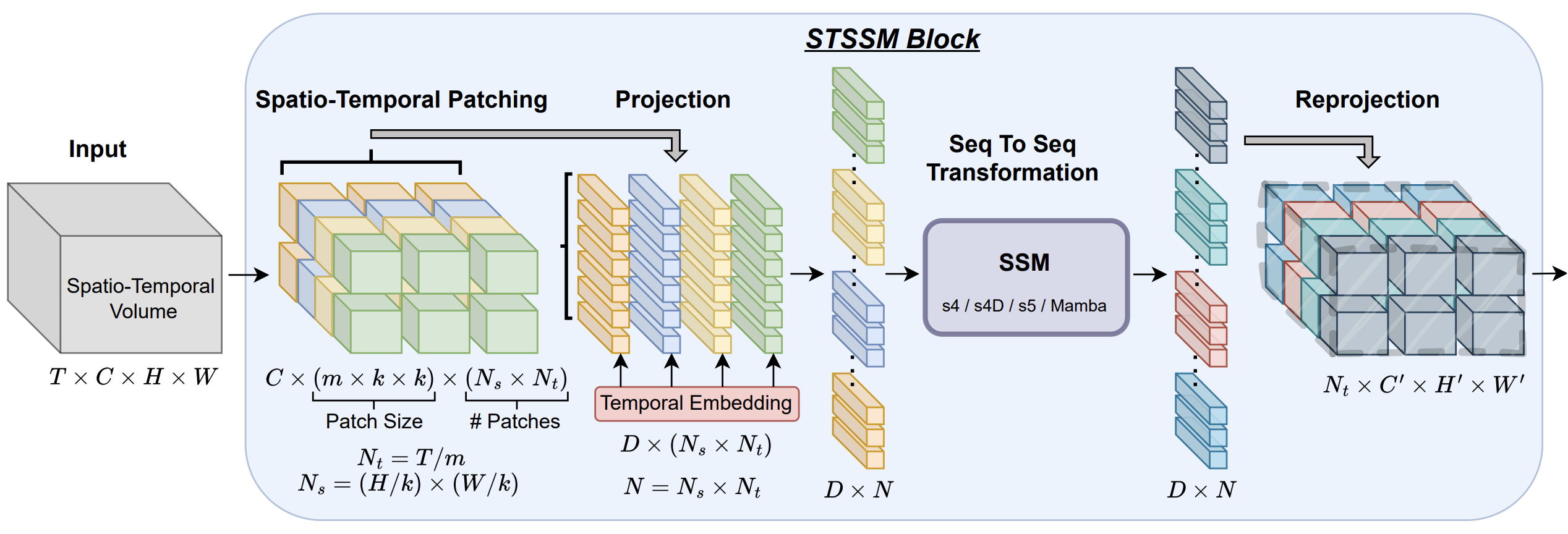
Next, we move up a level and begin building the STSSM block, which will become the central component of our event-driven model. The new CNeuronSpikeSTSSM object brings together everything implemented so far — the embedding stack and SSM modules — into a single structure capable of processing complete spatio-temporal market patterns.
class CNeuronSpikeSTSSM   :  public CNeuronSpikeConvBlock
  {
protected:
   CNeuronSpikePatchStak   cEmbedings;
   CLayer                  cProjection;
   CLayer                  cSSM;
   //---
   virtual bool      feedForward(CNeuronBaseOCL *NeuronOCL) override;
   virtual bool      calcInputGradients(CNeuronBaseOCL *NeuronOCL) override;
   virtual bool      updateInputWeights(CNeuronBaseOCL *NeuronOCL) override;

public:
                     CNeuronSpikeSTSSM(void) {};
                    ~CNeuronSpikeSTSSM(void) {};
   //---
   virtual bool      Init(uint numOutputs, uint myIndex, COpenCLMy *open_cl,
                          uint stack_size, uint dimension, uint patch_dimension,
                          uint ssm_dimension, uint variables,
                          ENUM_OPTIMIZATION optimization_type, uint batch);
   //---
   virtual int       Type(void)   override const   {  return defNeuronSpikeSTSSM;   }
   //--- methods for working with files
   virtual bool      Save(int const file_handle) override;
   virtual bool      Load(int const file_handle) override;
   //---
   virtual void      SetOpenCL(COpenCLMy *obj)   override;
   virtual void      TrainMode(bool flag) override;
   //---
   virtual bool      WeightsUpdate(CNeuronBaseOCL *source, float tau) override;
  };
Within the class, the key component is cEmbedings, our embedding stack, which prepares the event stream by creating a multidimensional representation of each market impulse. It is as if the trader were not just watching the price and volume, but were mapping out all the market signals from the past few seconds, identifying the relationships between them.
Next comes cProjection, which carefully distributes and transforms the embeddings, ensuring consistency between local patterns and the global market picture. This projects information into a space where the model can simultaneously analyze short-term fluctuations and long-term trends.
At the next level, cSSM comes into play — a stack of SSM modules that process complex temporal and spatial dependencies. It tracks how local market events combine to form general patterns, generating predictive signals. If we view the market as a living system, cSSM sees the movement of all streams simultaneously, linking short-term spikes to global trends.
The initialization method can be viewed as preparing an entire analytics center for market analysis. First, a foundational block is created — the base CNeuronSpikeConvBlock — which sets the internal dimensions.
bool CNeuronSpikeSTSSM::Init(uint numOutputs, uint myIndex, COpenCLMy *open_cl,
                             uint stack_size, uint dimension, uint patch_dimension,
                             uint ssm_dimension, uint variables,
                             ENUM_OPTIMIZATION optimization_type, uint batch)
  {
   if(!CNeuronSpikeConvBlock::Init(numOutputs, myIndex, open_cl, ssm_dimension * (stack_size - 2),
             ssm_dimension * (stack_size - 2), dimension, variables, 1, optimization_type, batch))
      return false;
Next, cEmbedings is initialized — an embedding stack that transforms each market event into a multidimensional signal. It's as if every candlestick, every trade, and every volume reading were transformed into a complex pattern that could be analyzed simultaneously across all parameters.
   uint index = 0;
   if(!cEmbedings.Init(0, index, OpenCL, stack_size, dimension, patch_dimension, variables, optimization, iBatch))
      return false;
The next level is cProjection. Here, the embeddings are carefully transformed and distributed across the analysis space so that the model can simultaneously capture short-term fluctuations and global market trends. Each layer in the projection acts as a kind of filter that identifies key patterns and prepares the data for the next step.
   cProjection.Clear();
   cProjection.SetOpenCL(OpenCL);
   CNeuronSpikeConvBlock* conv = NULL;
   index++;
   conv = new CNeuronSpikeConvBlock();
   if(!conv ||
      !conv.Init(0, index, OpenCL, 2 * patch_dimension, patch_dimension, patch_dimension,
                                      stack_size - 1, variables, optimization, iBatch) ||
      !cProjection.Add(conv))
     {
      DeleteObj(conv)
      return false;
     }
   index++;
   conv = new CNeuronSpikeConvBlock();
   if(!conv ||
      !conv.Init(0, index, OpenCL, 2 * patch_dimension, patch_dimension, ssm_dimension,
                                      stack_size - 2, variables, optimization, iBatch) ||
      !cProjection.Add(conv))
     {
      DeleteObj(conv)
      return false;
     }
At the top level, cSSM comes into play; it consists of two CNeuronSpikeMamba2D blocks. They aggregate all the information from embeddings and projections, capturing complex spatio-temporal relationships. You can think of them as analysts who take all the local signals and piece together an overall picture of the market by combining short-term impulses with long-term trends.
   cSSM.Clear();
   cSSM.SetOpenCL(OpenCL);
   CNeuronSpikeMamba2D* ssm = NULL;
   for(int i = 0; i < 2; i++)
     {
      index++;
      ssm = new CNeuronSpikeMamba2D();
      if(!ssm ||
         !ssm.Init(0, index, OpenCL, ssm_dimension, ssm_dimension, (stack_size - 2)*variables,
                                                                      optimization, iBatch) ||
         !cSSM.Add(ssm))
        {
         DeleteObj(ssm)
         return false;
        }
     }
//---
   return true;
  }
The initialization method ensures that all components are properly initialized, interconnected, and ready for parallel data processing. Market information can now flow through embeddings, projections, and SSM modules, forming a structured and coherent representation of the event space. Thus, the CNeuronSpikeSTSSM object is fully ready for training and analyzing real financial data streams, providing a stable foundation for subsequent calculations and forecasts.
The forward pass algorithm functions as a well-coordinated, multi-level analytical system, in which each stage carefully amplifies and refines the market signal as it passes through the model.
bool CNeuronSpikeSTSSM::feedForward(CNeuronBaseOCL *NeuronOCL)
  {
//---
   if(!cEmbedings.FeedForward(NeuronOCL))
      return false;
The forward pass begins when the data to be analyzed is fed into cEmbedings. This module transforms a raw stream of observations into a dense representation enriched with local spatio-temporal features. This is where the initial market structure takes shape, to be expanded and refined in subsequent stages.
Control is then passed to the cProjection chain. Each of its elements sequentially receives a signal from the previous layer and performs its own transformation.
   CNeuronBaseOCL* prev = cEmbedings.AsObject();
   CNeuronBaseOCL* curr = NULL;
   for(int i = 0; i < cProjection.Total(); i++)
     {
      curr = cProjection[i];
      if(!curr ||
         !curr.FeedForward(prev))
         return false;
      prev = curr;
     }
This is similar to how a signal moves through a hierarchy of indicators: first, the basic patterns are extracted, then the more complex relationships, and with each step, the data becomes clearer and more meaningful. With each layer, the model gains a more accurate understanding of the current context.
After projection, the data is fed into the cSSM block, which consists of two independent spatio-temporal modules. Each module receives a stream from the projection block, computes its own SSM representation, and then carefully combines the result with the input signal using a normalized summation operation. This step serves as a kind of stabilization mechanism: the model takes into account both the current state and the calculated dynamic changes. As a result, the forward pass becomes much more stable, especially when dealing with volatile data.
   uint units = GetUnits() * GetVariables();
   for(int i = 0; i < cSSM.Total(); i++)
     {
      curr = cSSM[i];
      if(!curr ||
         !curr.FeedForward(prev) ||
         !SumAndNormilize(curr.getOutput(), prev.getOutput(), curr.getOutput(),
                                     curr.Neurons() / units, true, 0, 0, 0, 1))
         return false;
      prev = curr;
     }
Finally, the updated signal is passed to the parent class, which aggregates all the received data and generates the final representation. This is the final stage, where all components of the architecture come together to create a comprehensive and refined picture of the market process.
   if(!CNeuronSpikeConvBlock::feedForward(prev))
      return false;
//---
   return true;
  }
The forward pass algorithm ensures a smooth and sequential transformation of data — from local patterns to global dynamics. Each step is performed with the previous one in mind, which makes the model robust against noise and capable of adapting to the actual pace of the financial market.
Thus, CNeuronSpikeSTSSM serves as the "brain" of the entire model. It accumulates the knowledge gained at previous levels, integrates it into a unified forecast, and ensures readiness for analysis and learning in any market scenario.
After such productive work, it is time to take a short break and let it all sink in. A short break will allow you to look at the project with fresh eyes and move forward with renewed energy. In the next article, we will reach the final stage: we will put the finishing touches on the architecture we have implemented and bring it to a logical conclusion.
Conclusion
The STSSM block we have optimized and its derivatives do not merely replicate the ideas of the framework's authors; they develop them further with a practical focus on real-world market challenges. During the implementation process, we did not limit ourselves to strictly following the original architecture. Key components were optimized for MQL5 and OpenCL, enabling high computational density and stable performance even with large time windows and a wide range of variables.
The main advantage of the STSSM approach is its ability to analyze temporal and spatial dynamics simultaneously. Our implementation makes this process particularly efficient through parallel computational threads, an improved normalization system, and a carefully designed projection-layer structure.
Thus, the resulting architecture combines the theoretical strength of the original framework with the practical applicability of our optimizations. We now have a flexible, scalable, and resource-efficient tool ready for testing under challenging financial market conditions.
Links
- Spatio-Temporal State Space Model for Efficient Event-Based Optical Flow
- Other articles in this series
Programs used in this article
| # | Name | Type | Description |
|---|---|---|---|
| 1 | Study.mq5 | Expert Advisor | Expert Advisor for offline model training |
| 2 | StudyOnline.mq5 | Expert Advisor | Online model training Expert Advisor |
| 3 | Test.mq5 | Expert Advisor | Model testing Expert Advisor |
| 4 | Trajectory.mqh | Class library | Data structure describing the system state and model architectures |
| 5 | NeuroNet.mqh | Class library | Class library for building a neural network |
| 6 | NeuroNet.cl | Library | Code library for an OpenCL program |
Translated from Russian by MetaQuotes Ltd.
Original article: https://www.mql5.com/ru/articles/20447
Warning: All rights to these materials are reserved by MetaQuotes Ltd. Copying or reprinting of these materials in whole or in part is prohibited.
This article was written by a user of the site and reflects their personal views. MetaQuotes Ltd is not responsible for the accuracy of the information presented, nor for any consequences resulting from the use of the solutions, strategies or recommendations described.