Neural Networks in Trading: Recurrent Modeling of Market Micromovements (Conclusion)

Introduction

The market remains that same complex, multi-layered system where every micro-event — whether a spike in volume or a shift in the liquidity balance — forms its own trajectory. We observe this fabric of events every day, but few architectural solutions are capable of handling it as naturally as an event-driven neural network does. That is precisely why the EV-MGRFlowNet framework has become the foundation for developing a truly modern approach to analyzing market micromovements. In previous articles, we examined the key elements of the original architecture and adapted them to the specific requirements of financial time series, porting them to the MQL5 environment using OpenCL. This approach is essential for achieving the ultimate goal — developing a model capable of perceiving the market as a stream of events in which the past and the present intertwine to form a single structure.

This perspective is closer to the classical interpretation of the behavior of a complex system, in which price change as a process takes center stage. It is here that the EV-MGRFlowNet architecture reveals its conceptual power. Its first major advantage is its ability to process data in event form, without requiring uniform sampling or fixed time windows. The market never moves at a steady pace: its rhythm is determined by surges of activity, lulls, and brief impulses, which, in the traditional approach, are lost between candlesticks. The event-driven model, on the other hand, reacts to every minor change as it occurs, rather than according to a predefined time grid, which makes it particularly expressive under actual price movement conditions.

Added to this is the depth of temporal memory provided by FERE-Net, which is based on ConvGRU and its modification, ST-ConvGRU. These mechanisms do more than simply collect information about the sequence of events. They maintain the structure of the unfolding movement, just as an experienced analyst tracks the overall kinematics of the process rather than momentary fluctuations. In a market where the direction of price movement is determined not by smooth trends but by chaotic bursts of liquidity, this memory becomes one of the architecture's key advantages. It is precisely because of this that the model does not lose context and can correctly interpret the sequence of market changes even when data density is high.

This dynamic is complemented by the multi-scale refinement implemented in FGD-Net. In the original architecture, it reconstructs optical flow at different resolution levels; in our financial context, it plays a similar role, allowing the model to reconstruct the direction and speed of market micromovements. This reconstruction views the market as a continuous vector process rather than a sequence of discrete points. Each new set of events refines the structure of the flow, creating a more coherent and stable description of the direction of movement. This makes it possible to analyze not only local spikes but also longer-lasting impulses. This is especially important for developing decision-making logic.

The HMC-Loss hybrid loss function plays an equally important role, as it allows the model to be trained without pre-prepared labels. For financial markets, where there is no single correct direction in the strict machine-learning sense, this property is crucial. The flow is assessed based on its internal temporal coherence, the smoothness of the reconstructed movement, and the internal connections between events. This approach naturally reduces the impact of random noise and highlights stable structures — the very ones that determine the actual dynamics of the market. Essentially, the model learns to distinguish between impulses that can develop into market movement and noise that should be ignored.

The authors’ visualization of the framework is shown below.

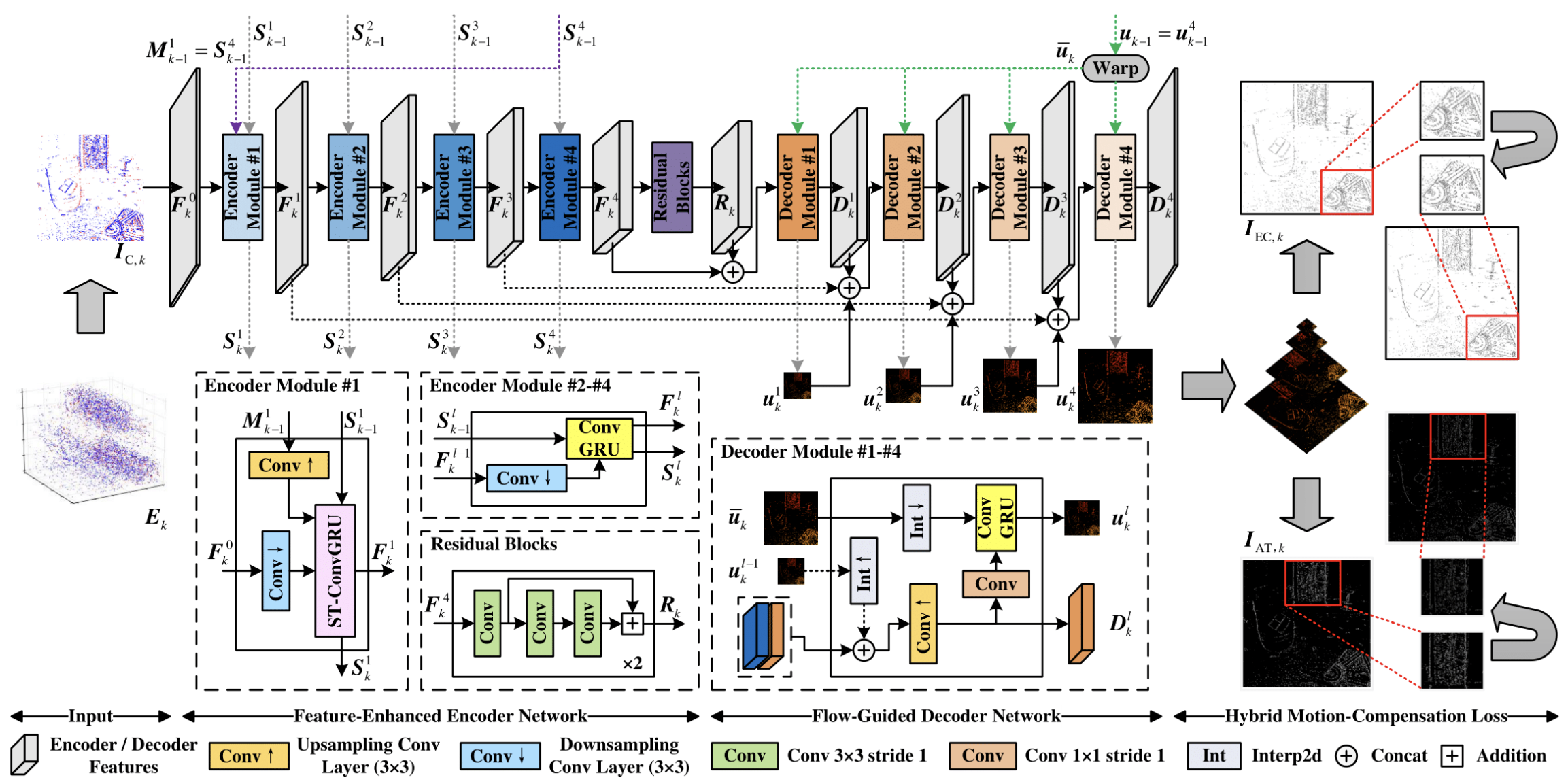
When porting the EV-MGRFlowNet architecture to MQL5, we faced not only the challenge of porting individual components but also the need to adapt the computational scheme itself. The implementation of ST-ConvGRU became the foundation upon which the entire framework is built. We have shown how to organize memory, how to maintain hidden states, and how to use OpenCL to process an event stream. These elements have formed a robust framework that enables the processing of large volumes of data while maintaining the architectural integrity of the model within a trading terminal environment.

A particular challenge was the absence of a spatial dimension in the financial data in the form typically used for computer vision tasks. Therefore, the multidimensionality of the original modules was reinterpreted through the structure of market data: event density, liquidity concentration, and the nature of aggressive and passive orders. This adaptation preserved the logic of the original architecture, allowing it to function in an environment where space is manifested not visually but structurally.

Today, we continue implementing the approaches proposed by the framework's authors using MQL5. At this stage, it is important for us not only to expand the architecture, but also to enable it to generate a meaningful description of market movements. While we previously focused on teaching the model to perceive the flow of events and maintain its structure through recurrent mechanisms, we are now taking the next step — moving on to reconstructing the market movement itself. This is precisely where the FGD-Net decoder comes into play — the very module that, in the original architecture, is responsible for multiscale refinement of the optical flow, and in our context becomes a tool for reconstructing the market dynamics vector.

Decoder

In the EV-MGRFlowNet architecture, the decoder plays a special role. It links the hidden states accumulated by the recurrent component to a specific prediction of the direction and intensity of motion, allowing the accumulated dynamics to be transformed into a form suitable for analysis. In other words, FGD-Net is a kind of lens through which the events collected by the model are transformed into a measurable and interpretable signal. That is exactly where we will begin our work today, examining the logic behind its design in detail and gradually adapting its architectural solutions to a format compatible with the capabilities of MQL5 and OpenCL.

Before we get started, let's take another look at the authors’ visualization of the decoder modules.

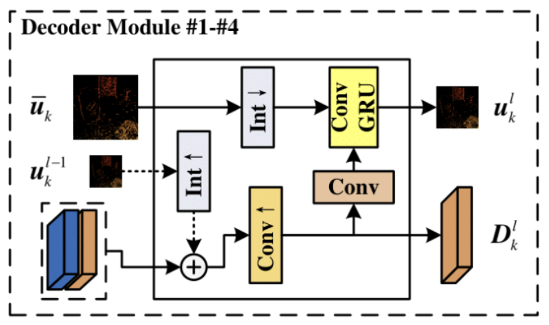
At first glance, it seems like just another iteration of a recurrent convolutional unit, but if you look more closely, it becomes clear that there is a much more subtle logic underlying the interaction between the model’s levels.

First and foremost, it is worth paying attention to how the features fed into the recurrent block are generated. Unlike the traditional architecture, in which each layer of the decoder operates exclusively on its own output or on the result from the previous layer, this approach uses a projection of a concatenated tensor that combines two sources of information. The first source is the output of the previous decoder layer — that is, the dynamics that have already been partially reconstructed at a lower resolution. The second is the corresponding encoder level, which contains structural information about the original events that has not yet been processed through the multiscale reconstruction mechanisms. This combination produces a structurally rich input signal that contains both accumulated context and up-to-date information about the spatial and structural characteristics of the events being analyzed.

This combination is not merely a technical device, but a fundamentally important element of the entire architecture. The model can refine its motion estimate by continuously comparing the current reconstruction with the actual structure of the original flow. In classical optical flow problems, this helps prevent drift and stabilize the velocity field. In our context, this allows us to adjust the market micromovement vector based on the actual event structure.

The organization of the hidden state is no less interesting. In a standard ConvGRU, it is updated layer by layer. Each level of the decoder stores and uses its own memory. Here, however, the approach is entirely different — the hidden state represents a projection of the entire model’s output from the previous step, rather than the local state of a single layer. This solution brings the decoder closer to the concept of a global recurrent mechanism. The model does not rely on partial, disjointed states, but instead uses a unified dynamic flow derived in the previous step of sequence processing. In this way, the architecture prevents errors from accumulating between layers and maintains a coherent historical trajectory within a single recurrent context.

That is exactly what makes FGD-Net so expressive. The decoder functions as a multi-stage filter that compares its intermediate reconstructions with the global state of the model at each step. This results in a reliable and stable reconstruction of the direction of motion — whether it is the optical flow in the original problem or the market microflow in our port.

And once the overall logic of the calculations becomes clear enough, the time comes to translate the architectural concept from an abstract diagram into a concrete object. This is where a new module comes into play, combining the functions of the decoder and integrating the separate computational branches into a single, functional structure. We are designing it as a standalone component of the model — flexible enough to process complex tensor structures, and rigorous enough to meet the requirements of OpenCL computations.

This is how the CNeuronFGDModule class is created, fitting neatly into the existing structure.

class CNeuronFGDModule  :  public CNeuronBaseOCL
  {
protected:
   CNeuronBatchNormOCL        cNorm;
   CNeuronConvOCL             cD;
   CNeuronBaseOCL             cFlowIn;
   CNeuronConvOCL             cFlow;
   CNeuronBaseOCL             cConcatenated;
   CNeuronMultiWindowsConvOCL cXH;
   //---
   virtual bool      GRU(void);
   virtual bool      GRU_grad(void);

   //---
   virtual bool      feedForward(CNeuronBaseOCL *NeuronOCL) override { return false; }
   virtual bool      feedForward(CNeuronBaseOCL *NeuronOCL, CBufferFloat *SecondInput)override;
   virtual bool      updateInputWeights(CNeuronBaseOCL *NeuronOCL) override { return false; }
   virtual bool      updateInputWeights(CNeuronBaseOCL *NeuronOCL, CBufferFloat *second)override;
   virtual bool      calcInputGradients(CNeuronBaseOCL *NeuronOCL) override { return false; }
   virtual bool      calcInputGradients(CNeuronBaseOCL *NeuronOCL,
                                        CBufferFloat *SecondInput,
                                        CBufferFloat *SecondGradient,
                                        ENUM_ACTIVATION SecondActivation = None) override;

public:
                     CNeuronFGDModule(void) {};
                    ~CNeuronFGDModule(void) {};
   //---
   virtual bool      Init(uint numOutputs, uint myIndex, COpenCLMy *open_cl, uint units,
                          uint main_dimension, uint flow_dimension, uint dimension_out,
                          ENUM_OPTIMIZATION optimization_type, uint batch);
   //---
   virtual int       Type(void)   override const   {  return defNeuronFGDModule;   }
   //--- methods for working with files
   virtual bool      Save(int const file_handle) override;
   virtual bool      Load(int const file_handle) override;
   //---
   virtual void      SetOpenCL(COpenCLMy *obj) override;
   //---
   virtual bool      WeightsUpdate(CNeuronBaseOCL *source, float tau) override;
   virtual CNeuronConvOCL* GetD(void)  { return cD.AsObject(); }
   virtual void      SetActivationFunction(ENUM_ACTIVATION value) override { };
  };

Its design reflects the same architectural concept that we observed in the decoder graph. Individual submodules are responsible for normalization, convolutional transformations, feature formation, and recurrent dynamics, while the main object acts as the coordinator of all interactions.

Initializing the object was a natural extension of the architectural logic. Here, the sizes of the input and output spaces are specified, the channel structure is defined, a connection to the OpenCL context is established, and optimization modes are set. The multilayered structure of the computational graph we discussed earlier is now taking physical form. Each component knows its place and its role, and each is ready to fit into the overall computation cycle.

bool CNeuronFGDModule::Init(uint numOutputs, uint myIndex, COpenCLMy *open_cl, uint units,
                            uint main_dimension, uint flow_dimension, uint dimension_out,
                            ENUM_OPTIMIZATION optimization_type, uint batch)
  {
   if(!CNeuronBaseOCL::Init(numOutputs, myIndex, open_cl, units * dimension_out,
                            optimization_type, batch))
      return false;
   activation = None;

As a first step, the module inherits the parameters of the base object. It is like the foundation on which the other components are built. Without a proper connection to the OpenCL context and correctly configured output channels, the rest of the logic simply cannot run. Next, top-level activation is disabled — it is important for the decoder to preserve purely numerical transformations without introducing nonlinearity where the framework's authors did not intend it.

Next, the step-by-step configuration of the internal components begins. We expect the module to receive a concatenated tensor at its input, formed from three data sources. Clearly, the values will have mismatched distributions, so we first use a batch normalization layer. It is responsible for aligning the scales of the feature maps.

   uint index = 0;
   if(!cNorm.Init(0, index, OpenCL, main_dimension * units, iBatch, optimization))
      return false;
   cNorm.SetActivationFunction(None);

Its initialization determines the number of channels, which is equal to the product of the main stream's dimension and the number of unitary sequences — the very space where the features of the encoder and decoder intertwine. The absence of an activation function underscores its modest yet indispensable role: it does not alter the meaning of the data, but merely ensures its stability for subsequent operations.

Next, the convolutional layer cD comes into play. This is a tool that introduces dynamics into the module — it maps the local state and generates refined motion maps. The TANH activation function was chosen deliberately. In the context of GRU, it helps keep values within a limited range, maintaining stability when updating the hidden state.

   index++;
   if(!cD.Init(0, index, OpenCL, main_dimension, main_dimension, dimension_out, units, 1, optimization, iBatch))
      return false;
   cD.SetActivationFunction(TANH);

Next, the flow projection block is initialized; it serves as a sort of gateway between the state of previous steps and the current computations.

   index++;
   if(!cFlowIn.Init(0, index, OpenCL, flow_dimension * units, optimization, iBatch))
      return false;
   DeleteObj(cFlowIn.getOutput())
   cFlowIn.SetActivationFunction(None);
   index++;
   if(!cFlow.Init(0, index, OpenCL, flow_dimension, flow_dimension, dimension_out, units, 1, optimization, iBatch))
      return false;
   cFlow.SetActivationFunction(None);

A little further on, a feature concatenation object (cConcatenated) is created. It is especially important here that the dimensions match exactly, because even the slightest discrepancy will instantly destroy the entire computational graph.

   index++;
   if(!cConcatenated.Init(0, index, OpenCL, 2 * dimension_out * units, optimization, iBatch))
      return false;
   cConcatenated.SetActivationFunction(None);

And the finishing touch — the multichannel convolution cXH. It serves as the computational core of the ConvGRU mechanism: this is where the projections of the analyzed features and the hidden state are generated. A pair of windows of the same size creates a symmetrical structure, and the total number of output channels — three times the width of the output dimension — reflects the three core elements of the GRU algorithm.

   index++;
   uint windows[] = { dimension_out, dimension_out };
   if(!cXH.Init(0, index, OpenCL, windows, 3 * dimension_out, units, 1, optimization, iBatch))
      return false;
   cXH.SetActivationFunction(None);
//---
   return true;
  }

No activation, no frills — just pure math.

Once all submodules have been initialized, the FGD module is now a unified architectural unit in which each element performs its own function, adhering to the order and structure established in the original model. And it is precisely this accuracy, this harmony of its internal structure, that makes it the foundation for the subsequent implementation of recurrent logic and the reconstruction of a multiscale motion field.

After initializing the object, we proceed to implement the forward pass algorithm in the feedForward method which follows the strict, deterministic data processing sequence characteristic of the EV-MGRFlowNet architecture.

bool CNeuronFGDModule::feedForward(CNeuronBaseOCL *NeuronOCL, CBufferFloat *SecondInput)
  {
   if(!cFlowIn.SetOutput(SecondInput, false))
      return false;

The module receives pointers to two sources of input data as parameters. One of them is represented by a buffer object. However, the architecture of the object's internal components calls for the use of only neural layers; therefore, as our first operation, we set the obtained pointer as the result buffer of a specially created object.

The next step is data normalization. The normalization layer evens out the distribution of input values, ensuring the stability of subsequent layers and improving training efficiency. An error at this stage causes the method to terminate immediately.

   if(!cNorm.FeedForward(NeuronOCL))
      return false;

After normalization, the data is passed to the cD block. This component acts as a transformation layer that performs convolutional filtering operations and generates an initial feature map.

   if(!cD.FeedForward(cNorm.AsObject()))
      return false;

In parallel, a second data stream is processed through cFlow, which projects the global hidden state into the feature space of the current layer.

   if(!cFlow.FeedForward(cFlowIn.AsObject()))
      return false;

Next, the results of both streams are concatenated.

   if(!Concat(cD.getOutput(), cFlow.getOutput(), cConcatenated.getOutput(),
              cD.GetFilters(), cFlow.GetFilters(), cFlow.GetUnits()))
      return false;

The combined data is passed to the cXH layer. It projects the features being analyzed and the hidden state into the quantities required to perform the operations of the GRU algorithm. Using the multi-window convolution object allows us to generate all these quantities simultaneously in parallel threads within the OpenCL context.

   if(!cXH.FeedForward(cConcatenated.AsObject()))
      return false;

A key step in the forward pass is the call to the GRU method, where recurrent processing of temporal dependencies takes place. The GRU enables the module to account for sequences of events over time, which is critical for analyzing financial data. Any error at this step stops the method.

   if(!GRU())
      return false;

Before the method completes, we set the gradients of the cD block to zero. This operation ensures that previously accumulated gradient values will not affect subsequent training iterations, keeping the computations clean.

   if(!cD.getGradient().Fill(0))
      return false;
//---
   return true;
  }

If all steps are completed successfully, the method returns true, confirming that the forward pass was executed correctly. Taken together, this sequence reflects the key principles of the EV-MGRFlowNet architecture: clear modularity, state control for each block, and optimization of computational resources.

The calcInputGradients method implements a key component of the training process for the CNeuronFGDModule module — the backpropagation algorithm. While the forward pass organizes the flow of information through the network, backpropagation is responsible for adjusting the parameters and allows the model to gradually converge toward the desired results.

bool CNeuronFGDModule::calcInputGradients(CNeuronBaseOCL *NeuronOCL,
                                          CBufferFloat *SecondInput,
                                          CBufferFloat *SecondGradient,
                                          ENUM_ACTIVATION SecondActivation = None)
  {
   if(!NeuronOCL || !SecondGradient)
      return false;

The method begins by verifying the validity of the pointers to the source data objects. Without them, further calculations are impossible. This is a basic but critically important safeguard against errors.

Next, we synchronize the pointers to the gradient buffer of the second data stream and a specially created internal object.

   if(!cFlowIn.SetGradient(SecondGradient, true))
      return false;
   cFlowIn.SetActivationFunction(SecondActivation);

Next, the error gradient is backpropagated through the recurrent block. This is where the gradients of the recurrent connections are computed, which allows us to account for the effect of temporal dependencies on the model's error.

   if(!GRU_grad())
      return false;

The next step is to compute the hidden gradients of the combined buffer. The method correctly distributes the error among the combined streams, preparing the data for separate processing.

   if(!cConcatenated.CalcHiddenGradients(cXH.AsObject()))
      return false;

The DeConcat operation splits the combined gradient into parts corresponding to the cD and cFlow layers. The filter parameters and sequence dimensionality ensure the correct partitioning of multidimensional data.

   if(!DeConcat(cD.getPrevOutput(), cFlow.getGradient(), cConcatenated.getGradient(),
                cD.GetFilters(), cFlow.GetFilters(), cFlow.GetUnits()))
      return false;

Next, the gradient of the cD object is summed. This step allows us to combine the values of the two data streams and stabilize the training process.

   if(!SumAndNormilize(cD.getGradient(), cD.getPrevOutput(), cD.getGradient(), cD.GetFilters(), false, 0, 0, 0, 1))
      return false;

The Deactivation method correctly adjusts the resulting gradient values using the derivatives of the corresponding activation functions.

   Deactivation(cFlow)
   Deactivation(cD)

Next, we correctly propagate the gradients of the two data streams back to the source data.

   if(!cFlowIn.CalcHiddenGradients(cFlow.AsObject()))
      return false;
   if(!cNorm.CalcHiddenGradients(cD.AsObject()))
      return false;
   if(!NeuronOCL.CalcHiddenGradients(cNorm.AsObject()))
      return false;
//---
   return true;
  }

If all steps were completed successfully, the method returns true, indicating that the gradients were calculated correctly.

Taken together, this sequence reflects fine-grained control over error distribution and demonstrates the modular, robust architecture of EV-MGRFlowNet, in which each component performs its specific task and ensures stable model training.

Thus, the FGD module becomes not just a part of the architecture, but also a bridge between theory and practice. It adopts the same structural choices as the original model, but expresses them in a form compatible with the MQL5 and OpenCL environments. And it is precisely at this stage that it becomes clear: the decoder is not just a formality, but the key to enabling the model to reconstruct motion in all its multiscale complexity.

Top-level object

Following the successful implementation of individual modules of the EV-MGRFlowNet framework, the next key step is to integrate all components into a single, cohesive structure. This role is fulfilled by the CNeuronEVMGRFlowNet class, which inherits basic functionality from CNeuronSpikeActivation and combines an encoder, a central block, and a decoder, providing a complete information processing cycle from the model’s input to its output.

class CNeuronEVMGRFlowNet  :  public CNeuronSpikeActivation
  {
protected:
   CNeuronFERENet                   cEncoder;
   CNeuronSTEFlowNetResidualBlock   cNeck;
   CLayer                           cDecoder;
   //---
   virtual bool      feedForward(CNeuronBaseOCL *NeuronOCL) override;
   virtual bool      updateInputWeights(CNeuronBaseOCL *NeuronOCL) override;
   virtual bool      calcInputGradients(CNeuronBaseOCL *NeuronOCL) override;

public:
                     CNeuronEVMGRFlowNet(void) {};
                    ~CNeuronEVMGRFlowNet(void) {};
   //---
   virtual bool      Init(uint numOutputs, uint myIndex, COpenCLMy *open_cl,
                          uint units, uint &chanels[],
                          ENUM_OPTIMIZATION optimization_type, uint batch);
   //---
   virtual int       Type(void)   override const   {  return defNeuronEVMGRFlowNet;   }
   //--- methods for working with files
   virtual bool      Save(int const file_handle) override;
   virtual bool      Load(int const file_handle) override;
   //---
   virtual void      SetOpenCL(COpenCLMy *obj) override;
   virtual bool      Clear(void) override;
   //---
   virtual bool      WeightsUpdate(CNeuronBaseOCL *source, float tau) override;
   virtual void      SetActivationFunction(ENUM_ACTIVATION value) override { };
  };

Within the class, we see three main components:

• cEncoder (CNeuronFERENet) — acts as a feature encoder and translates the analyzed data into the model's internal representation;
• cNeck (CNeuronSTEFlowNetResidualBlock) — serves as the central residual processing block, enabling deep extraction and transformation of hidden features;
• cDecoder — maps the transformed representation back into the output data space.

This division illustrates the modular approach of EV-MGRFlowNet, in which each block is responsible for a strictly defined task, and their integration ensures the coordinated operation of the entire model.

The Init method performs a comprehensive initialization of all the class's internal components, ensuring structural consistency and correct model operation at every level. This is a key step in building the complete architecture — from the encoder to the decoder — ready for training and a forward pass.

bool CNeuronEVMGRFlowNet::Init(uint numOutputs, uint myIndex, COpenCLMy *open_cl,
                               uint units, uint &chanels[],
                               ENUM_OPTIMIZATION optimization_type, uint batch)
  {
   if(chanels.Size() < 2)
      return false;
   if(!CNeuronSpikeActivation::Init(numOutputs, myIndex, open_cl, units * chanels[0], optimization_type, batch))
      return false;

First, the method checks that the input channel array chanels is valid — the array must contain at least two elements. This ensures that the network will have both incoming and outgoing data flows. If the condition is not met, initialization is aborted.

Next, the method of the same name in the parent class is called to initialize the basic functionality and configure the object's fundamental settings, including resource allocation and memory for computations.

The number of layers in the encoder and decoder is set to one less than the number of elements in the channel array.

   uint layers = chanels.Size() - 1;

Next, the encoder is created and initialized. It receives the parameters provided by the user.

//--- Encoder
   int index = 0;
   if(!cEncoder.Init(0, index, OpenCL, units, chanels, optimization, iBatch))
      return false;

Successful initialization of the encoder ensures that the internal data representation is formed correctly.

The next step is to initialize the central block cNeck, which is responsible for deep feature extraction and provides the residual connections necessary for stable training of the deep model.

   index++;
   if(!cNeck.Init(0, index, OpenCL, chanels[layers], units, 32, 8, optimization, iBatch))
      return false;

Next, let's move on to working with the decoder. First, the dynamic array of objects is cleared and a pointer to the OpenCL object is passed; then, the construction of the data reconstruction layers begins.

//--- Decoder
   cDecoder.Clear();
   cDecoder.SetOpenCL(OpenCL);
   CNeuronFGDModule* fgd = NULL;
   CNeuronBaseOCL*   concat = cNeck.AsObject();
   uint flow_dimension = chanels[0];

At each stage, a new CNeuronFGDModule is created with parameters corresponding to the dimensions of the previous layer (main_dimension), the flow size (flow_dimension), and the number of outputs of the current layer. After successful initialization, the module is added to the decoder.

   for(uint i = 0; i < layers; i++)
     {
      uint main_dimension = concat.Neurons() / units;
      fgd = new CNeuronFGDModule();
      if(!fgd ||
         !fgd.Init(0, index, OpenCL, units, main_dimension, flow_dimension, chanels[layers - i - 1],
                                                                            optimization, iBatch) ||
         !cDecoder.Add(fgd))
        {
         DeleteObj(fgd)
         return false;
        }

Special attention has been paid to ensuring that the layers are combined correctly. If a corresponding encoder layer exists for the current level, a concat object is created that concatenates the neurons from the decoder, block D of the current module, and the encoder.

      if(i == (layers - 1))
         break;
      index++;
      CNeuronBaseOCL* encoder = cEncoder.GetLayer(-int(i + 1));
      CNeuronBaseOCL* d = fgd.GetD();
      if(!encoder)
        {
         concat = new CNeuronBaseOCL();
         if(!concat ||
            !concat.Init(0, index, OpenCL, fgd.Neurons() + d.Neurons(), optimization, iBatch) ||
            !cDecoder.Add(concat))
           {
            DeleteObj(concat)
            return false;
           }
        }
      else
        {
         concat = new CNeuronBaseOCL();
         if(!concat ||
            !concat.Init(0, index, OpenCL, fgd.Neurons() + d.Neurons() + encoder.Neurons(), optimization, iBatch) ||
            !cDecoder.Add(concat))
           {
            DeleteObj(concat)
            return false;
           }
        }
      index++;
     }

If there is no encoder, concatenation is performed only between the decoder and block D. This mechanism ensures the consistent propagation of signals and gradients across levels, preserving the integrity of the architecture.

After all the decoder layers have been built, a normalization layer is added. It stabilizes the distribution of activations, minimizes bias, and speeds up training, which is especially important when working with deep neural networks.

   CNeuronBatchNormOCL* norm = new CNeuronBatchNormOCL();
   if(!norm ||
      !norm.Init(0, index, OpenCL, fgd.Neurons(), iBatch, optimization) ||
      !cDecoder.Add(norm))
     {
      DeleteObj(norm)
      return false;
     }
//---
   return true;
  }

If an error occurs at any step, the method immediately terminates, freeing up resources. If all components are successfully initialized, the method returns true, indicating that the model is fully ready for training and a forward pass.

Once all of the object's components have been initialized, the next step is to construct a forward pass algorithm that ensures the sequential processing of the input data through the encoder, the central block, and the decoder. The feedForward method implements this process, ensuring coordinated signal propagation.

bool CNeuronEVMGRFlowNet::feedForward(CNeuronBaseOCL *NeuronOCL)
  {
   if(!cEncoder.FeedForward(NeuronOCL))
      return false;

First, the data passes through an encoder, which constructs an internal representation of the analyzed signals by extracting primary features and organizing them into a multidimensional space of latent representations. Any error at this step immediately terminates the method, preventing incorrect processing.

The signal is then sent to the central block cNeck. This residual block is responsible for the deep transformation of features, ensuring the model's stability and the effective extraction of complex relationships among the source data.

   if(!cNeck.FeedForward(cEncoder.AsObject()))
      return false;

Next, the decoder begins processing. The number of layers is defined as half the total number of elements in the decoder, reflecting the alternating arrangement of reconstruction modules and intermediate buffers. For each layer, pointers are created to the current FGD module, the D block, the corresponding encoder layer (encoder), and the previous layer (prev), ensuring precise control of data flows.

//--- Decoder
   int layers = cDecoder.Total() / 2;
   CNeuronFGDModule* fgd = NULL;
   CNeuronBaseOCL*   d = NULL;
   CNeuronBaseOCL*   encoder = NULL;
   CNeuronBaseOCL*   prev = cNeck.AsObject();
   CNeuronBaseOCL*   flow = cDecoder[-2];
   if(!flow.SwapOutputs())
      return false;
   uint units = cEncoder.GetUnits();
   if(!flow)
      return false;

Special attention is paid to preparing the output stream from the previous layer, which ensures that information is correctly passed through the decoder.

At each level of the decoder, the forward pass method of the corresponding FGD module is called, and the module receives data from the previous layer and an additional stream.

   for(int i = 0; i < layers; i++)
     {
      fgd = cDecoder[i * 2];
      if(!fgd ||
         !fgd.FeedForward(prev, flow.getPrevOutput()))
         return false;

The data is then combined with the outputs of the corresponding encoder layers and the D block using the Concat method, which ensures dimensional consistency and correctly merges the multidimensional data.

      prev = cDecoder[i * 2 + 1];
      if(!prev)
         return false;
      if(i == (layers - 1))
        {
         if(!prev.FeedForward(fgd))
            return false;
         break;
        }
      d = fgd.GetD();
      encoder = cEncoder[-(i + 1)];
      if(!encoder)
        {
         if(!Concat(fgd.getOutput(), d.getOutput(), prev.getOutput(),
                    fgd.Neurons() / units, d.Neurons() / units, units))
            return false;
        }
      else
        {
         if(!Concat(fgd.getOutput(), d.getOutput(), encoder.getOutput(), prev.getOutput(),
                    fgd.Neurons() / units, d.Neurons() / units, encoder.Neurons() / units, units))
            return false;
        }
     }

In the final layer, a forward pass is performed through the intermediate buffer prev, after which the results are passed to the method of the same name in the parent class, completing the full processing cycle.

   return CNeuronSpikeActivation::feedForward(prev);
  }

This ensures that the signal has been fully processed and is ready for the next stage.

The next step after the forward pass is to process errors and distribute gradients across all levels of the model. The calcInputGradients method implements backpropagation for the entire EV-MGRFlowNet architecture, ensuring that the weights are updated correctly and the model is prepared for the next iteration.

bool CNeuronEVMGRFlowNet::calcInputGradients(CNeuronBaseOCL *NeuronOCL)
  {
   if(!NeuronOCL)
      return false;

First, a basic check is performed on the received pointer to the source data object. If the object does not exist, further calculations are not possible, and the method immediately returns false.

Next, the method of the same name in the parent class is called to pass the gradients to the decoder's final layer, which completes the forward-pass chain.

   if(!CNeuronSpikeActivation::calcInputGradients(cDecoder[-1]))
      return false;

The decoder is processed in reverse order. The number of layers is calculated as half the total number of elements in the dynamic array.

//--- Decoder
   int layers = cDecoder.Total() / 2;
   CNeuronFGDModule* fgd = cDecoder[-2];
   CNeuronBaseOCL*   d = NULL;
   CNeuronBaseOCL*   encoder = NULL;
   CNeuronBaseOCL*   next = cDecoder[-1];
   CNeuronBaseOCL*   flow = cDecoder[-2];
   if(!fgd ||
      !fgd.CalcHiddenGradients(next))
      return false;
   uint units = cEncoder.GetUnits();

At each level, pointers are created to the current FGD module, the D block, the corresponding encoder layer (encoder), the next object (next), and the stream (flow).

In the first stage of the decoder's backward pass, the error is propagated to the FGD module. Next, in the loop, gradients are computed for each layer of the decoder, starting with the second-to-last layer and moving toward the input.

   for(int i = layers - 2; i >= 0; i--)
     {
      next = cDecoder[i * 2 + 1];
      if(!next ||
         !next.CalcHiddenGradients(fgd, flow.getOutput(), flow.getGradient(), (ENUM_ACTIVATION)flow.Activation()))
         return false;
      //---
      fgd = cDecoder[i * 2];
      if(!fgd)
         return false;
      d = fgd.GetD();
      encoder = cEncoder[-(i + 1)];

Particular attention is paid to the DeConcat operation, which splits the concatenated gradients into their components for the FGD module, the D block, and, if present, the corresponding encoder layer. This approach ensures dimensional consistency and the proper distribution of error across the layers.

      if(!encoder)
        {
         if(!DeConcat(fgd.getGradient(), d.getGradient(), next.getGradient(),
                      fgd.Neurons() / units, d.Neurons() / units, units))
            return false;
        }
      else
        {
         if(!DeConcat(fgd.getGradient(), d.getGradient(), encoder.getGradient(), next.getGradient(),
                      fgd.Neurons() / units, d.Neurons() / units, encoder.Neurons() / units, units))
            return false;
        }
      Deactivation(fgd);
     }

After the gradients for each FGD module are calculated, the resulting values are adjusted using the derivative of the corresponding activation function.

The final stage of error propagation passes through the central block cNeck and the encoder cEncoder.

   if(!cNeck.CalcHiddenGradients(fgd, flow.getOutput(), flow.getGradient(), (ENUM_ACTIVATION)flow.Activation()))
      return false;
   if(!cEncoder.CalcHiddenGradients(cNeck.AsObject()))
      return false;
   if(!NeuronOCL.CalcHiddenGradients(cEncoder.AsObject()))
      return false;
//---
   return true;
  }

Finally, the input data object receives the gradients from the encoder, which completes the full backpropagation cycle.

If all operations are completed successfully, the method returns true. Taken together, this algorithm demonstrates a carefully designed sequence of error propagation and gradient control, ensuring stable training of the EV-MGRFlowNet model and maintaining consistency across all internal data flows.

Overall, CNeuronEVMGRFlowNet serves as the link between all components of EV-MGRFlowNet. Its architecture reflects the classic principles of modularity and control, while retaining the ability to perform in-depth analysis and processing of temporal dependencies, making the model flexible, robust, and effective for forecasting tasks based on financial data.

Now that the key approaches proposed by the authors of the EV-MGRFlowNet framework have been implemented, it is important to highlight the architectural features of the models being trained. In this project, we are building a fully-fledged trading system capable of making decisions and executing trades in the financial market autonomously.

All architectural decisions were carried over from previous work with virtually no changes, which made it possible to retain the time-tested signal processing logic and learning algorithms. The main changes were made to the environment state encoder. That is where the top-level object CNeuronEVMGRFlowNet was integrated as a separate layer. This approach minimizes the complexity of integrating the framework into the model, while preserving the modularity and cleanliness of the architecture, and also simplifies future maintenance and expansion of the model.

Creating a top-level object serves as a bridge of sorts between the base modules and the external model, ensuring coordinated interaction among all layers without the need for a major overhaul of the existing structure. This solution reflects the core principle of EV-MGRFlowNet: high modularity with minimal integration effort.

The complete code describing the architecture of the models being trained is provided in the attachment.

Testing

Now that the EV-MGRFlowNet framework has been integrated into the environment state encoder, our model is ready to enter its first training arena. This stage can be compared to a novice trader practicing with historical data. The model receives a map of past market conditions, studies price movements, and tries to understand how to act in different situations.

Imagine that EURUSD from January 2024 through June 2025 is its training ground. Like a novice trader, the model examines each candlestick, analyzes trading volume, and looks for hidden patterns among key features. And EV-MGRFlowNet is its mentor: it points out what to focus on, creates an informative state representation for the Actor and the Critic, and helps it develop a trader’s intuition. With each step, it learns to predict market movements and assess risks, gradually progressing from a student to a confident trainee.

The next step is real-time online training using the MetaTrader 5 Strategy Tester. The luxury of calmly working with historical data is now gone. Each candlestick is like a real-time market reaction. The model reacts instantly, analyzes fluctuations caused by noise, adapts to sudden spikes, and adjusts its actions during periods of low liquidity. EV-MGRFlowNet acts as an invisible mentor, keeping the network from making mistakes and advising it when to act boldly and when to exercise caution. The underlying structure, built on historical data, remains its foundation, but the model now learns to respond flexibly to the current situation, much like a trader with live trading experience.

The final exam is testing the model on new data from July through September 2025. All the skills acquired in the previous stages are put to the test: no hints, just the market and its own decisions. The test results are presented below.

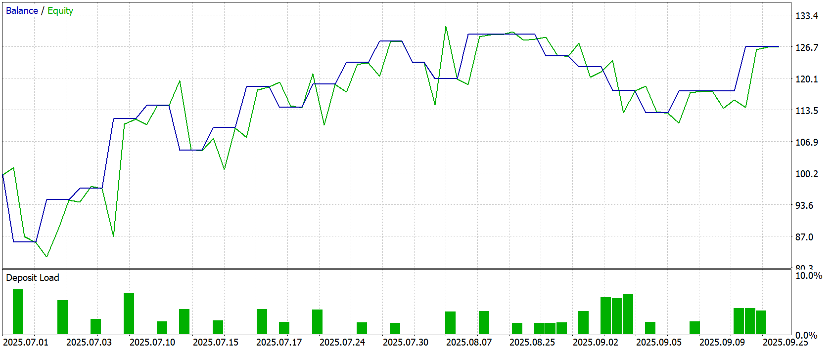
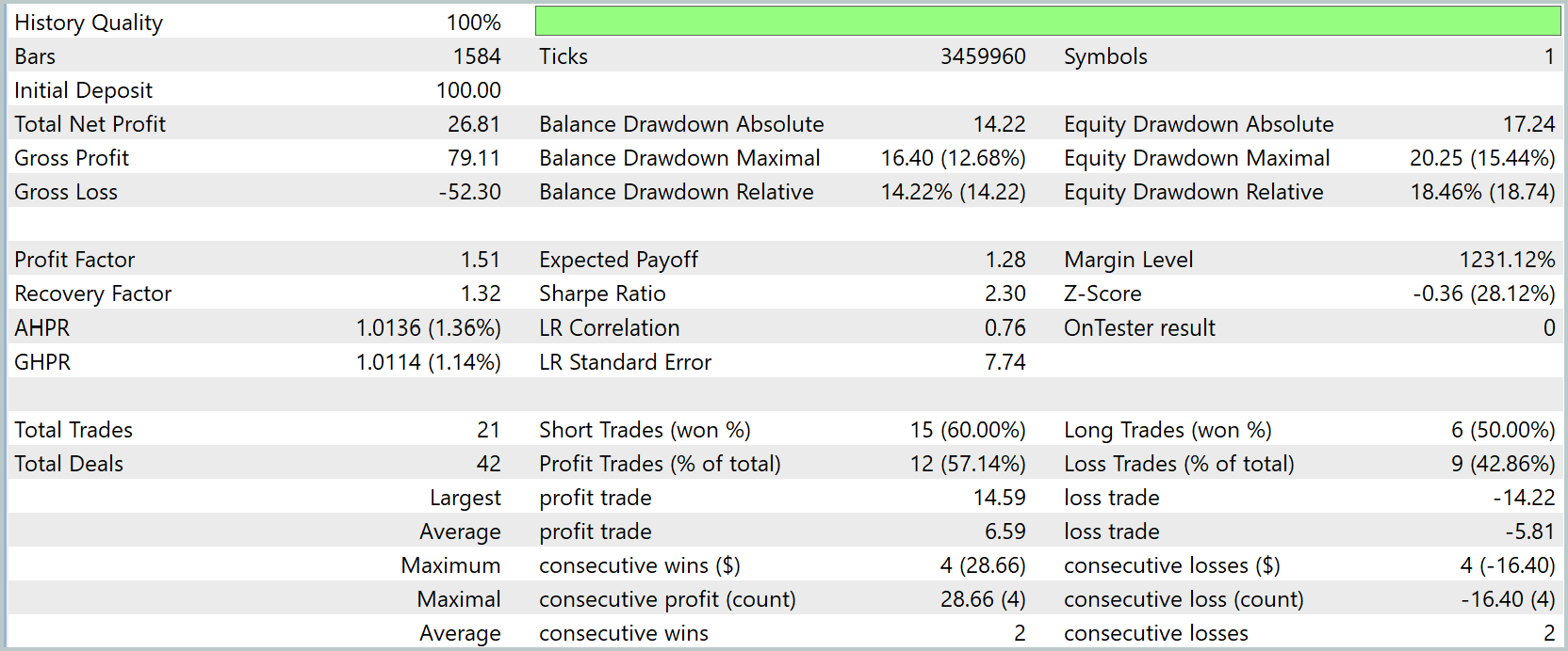
The test results show steady, stable performance. The equity curve rises steadily, without sharp spikes or erratic fluctuations. The balance and equity move almost in tandem, as if they were two coordinated mechanisms. One supports the strategy's underlying logic, while the other reflects the current status of open positions. Together, they produce smooth growth that feels neither random nor forced. The resulting growth — from USD 100.0 to USD 126.81 — appears to be a natural outcome of the algorithm's operation, rather than a consequence of random fluctuations.

This smoothness is supported by quantitative data. A profit factor of 1.51 and a recovery factor of 1.32 indicate that the strategy not only generates profits more often than losses, but also recovers steadily from drawdowns. The average profit per trade of USD 1.28 is not generated by isolated spikes but through consistent, steady movement, which makes the outcome more predictable.

Drawdowns are viewed as natural fluctuations. The maximum balance drawdown of USD 16.40 (12.68%) and maximum equity drawdown of USD 20.25 (15.44%) are not cause for concern, since the equity hardly deviates from the balance. This means that open positions do not remain in the red or place a prolonged strain on margin, and the chart clearly shows that small declines are quickly followed by consecutive gains.

The trading structure demonstrates the algorithm's internal harmony. Of the 21 trades, about 57% were profitable, and the distribution of short and long positions appears balanced. This indicates that the strategy is not fixated on a single market phase and can adapt to various conditions, whether momentum moves or periods of sideways trading.

Monitoring the equity curve and deposit load shows disciplined trading with a low leverage ratio. The deposit load rarely exceeds a few percent and generally remains within the 1–5% range. The algorithm does not take an overly aggressive approach to the market; it acts decisively, but within the defined risk limits.

Ultimately, the backtesting reveals a comprehensive, consistent picture: the algorithm steadily grows the capital, keeps drawdowns under control, and consistently generates profits.

Conclusion

We have completed the implementation of the approaches proposed by the authors of the EV-MGRFlowNet framework. The implemented solution demonstrates a high degree of architectural coherence, resilience to market fluctuations, and the ability to develop strategies independently. Integrating all components — the encoder, the central unit, and the decoder — into a single structure has made it possible to create a model that manages capital smoothly and predictably, minimizing stressful drawdowns and maintaining control over risks.

Testing showed that the strategy performs in a balanced manner. Profits are generated systematically, without relying on isolated successful trades, and backpropagation mechanisms ensure that the weights are consistently updated and that the model remains adaptive. The profit factor, recovery factors, and geometric return metrics confirm the effectiveness and reliability of the model.

The main advantage of the solution is its modularity and flexibility. The top-level object CNeuronEVMGRFlowNet can be easily integrated into various trading models while preserving the proven operational logic of all layers. This makes the framework not only a powerful tool for analysis and forecasting, but also a platform for further optimizing strategies, improving adaptability, and expanding functionality.

Links

• EV-MGRFlowNet: Motion-Guided Recurrent Network for Unsupervised Event-Based Optical Flow with Hybrid Motion-Compensation Loss
• Other articles in this series

Software used in this article

#	Name	Type	Description
1	Study.mq5	Expert Advisor	Expert Advisor for offline model training
2	StudyOnline.mq5	Expert Advisor	Expert Advisor for online model training
3	Test.mq5	Expert Advisor	Expert Advisor for model testing
4	Trajectory.mqh	Class library	Structure for describing the system state and model architectures
5	NeuroNet.mqh	Class library	Class library for building a neural network
6	NeuroNet.cl	Library	Code library for an OpenCL program