A Grid Expert Advisor Based on a Cellular Automaton with Online Learning in MQL5 (Part III): A Living Feature Graph
 279
 0

A Trainable Feature Graph: When the Connections Between Market Factors Come to Life
In the previous part of this series, we converted the Cellular10K architecture from a conventional grid to a graph structure. The features are no longer just an array, feat[50], and the cells of the cellular automaton now have not only geometric neighborhoods but also logical connections based on features, strategies, and long-range small-world chords. This was an important step: the model began to think not in terms of a flat grid, but in terms of a network of interacting agents.
However, a fixed graph has a fundamental limitation. If we specify in advance that momentum is connected to trend strength, RSI to Bollinger Bands, and volatility to ATR, we are once again introducing a rigid assumption into the system. Yes, it is smarter than a regular grid, but it is still static. The market, however, is constantly changing: today, volume confirms a breakout; tomorrow, that same volume turns out to be a trap; today, the RSI acts as a reversal indicator; tomorrow, it simply shows the strength of the trend.
For this reason, the third step in developing the architecture is to make the graph trainable rather than fixed. Now, the connections between features are strengthened if, taken together, they lead to a profitable prediction, and weakened if their combined effect leads to an error. As a result, the system gains not only 10,000 adaptive cells but also a dynamic feature-space structure.
The Main Idea: Not Neural Network Weights, but Connections between Causes
A conventional neural network learns the weights between neurons. In the third version of Cellular10K, both the cells and the connections between market features are trained. This is a fundamentally different level of adaptation.
A feature on its own rarely has a stable meaning. Momentum without volatility may just be noise. RSI without the context of the price's position within the channel may give a false signal. Volume, taken out of the context of the trend, can indicate either accumulation or distribution. Therefore, in real-world trading, it is not individual features that matter, but rather their effective combinations.
The trainable feature graph answers the question: "Which features in the current market regime actually reinforce each other, and which ones merely add noise?"
To do this, a connection matrix is introduced:
double m_fgraph[CNN_FEATURES * CNN_FEATURES]; // 50 × 50 trainable feature-to-feature connections
If m_fgraph[0][5] is increasing, it means that short-term momentum and short-term trend strength have often jointly produced correct predictions. If m_fgraph[16][22] falls, it means that the RSI14 + Bollinger20 combination is no longer functioning as a reliable reversal pattern in the current market regime.
Graph Initialization: A Soft Structure Instead of Random Chaos
The trainable graph should not start out completely random. If all connections are zero, the model will spend too much time on initial self-organization. If the connections are too strong, the model will become dogmatic. Therefore, soft initialization is used: local connections between features are assigned a small positive weight, while distant small-world connections are assigned an even smaller weight.
//+------------------------------------------------------------------+
//| Initialization of the trainable feature graph                    |
//+------------------------------------------------------------------+
void InitLearnableFeatureGraph()
  {
   for(int i = 0; i < CNN_FEATURES; i++)
     {
      for(int j = 0; j < CNN_FEATURES; j++)
        {
         double w = 0.0;

         //--- Local proximity of features: momentum next to momentum, RSI next to RSI
         if(MathAbs(i - j) == 1)
            w = 0.08;

         //--- distant small-world chord: the feature is assigned a weak connection to a distant group
         int chord = (i * 17 + 11) % CNN_FEATURES;
         if(j == chord)
            w = 0.04;

         //--- Self-loops are prohibited so that a feature does not reinforce itself indefinitely
         if(i == j)
            w = 0.0;

         m_fgraph[i * CNN_FEATURES + j] = w;
        }
     }
  }
This is similar to the biological nervous system: at birth, the connections are already there, but their strength is not yet fully established. From there, the market itself shows which connections are useful and which ones should wither away.
Feature Graph Layer
The graph layer is applied after the 50 base features have been calculated. It does not replace the features, but rather passes information from neighboring features through them, taking into account the current connection strength.
//+------------------------------------------------------------------+
//| Feature graph layer (one message-passing step)                   |
//+------------------------------------------------------------------+
void ApplyLearnableFeatureGraph(double &feat[])
  {
   double src[CNN_FEATURES];
   double dst[CNN_FEATURES];

   for(int i = 0; i < CNN_FEATURES; i++)
     {
      src[i] = feat[i];
      dst[i] = feat[i] * 0.72; // The feature's own voice remains the most important
     }

   for(int i = 0; i < CNN_FEATURES; i++)
     {
      double acc  = 0.0;
      double norm = 0.0;

      for(int j = 0; j < CNN_FEATURES; j++)
        {
         if(i == j)
            continue;

         double w = m_fgraph[i * CNN_FEATURES + j];
         if(MathAbs(w) < 0.0001)
            continue;

         acc  += src[j] * w;
         norm += MathAbs(w);
        }

      if(norm > 0.0001)
         dst[i] += 0.28 * acc / norm;
     }

   for(int i = 0; i < CNN_FEATURES; i++)
      feat[i] = MathTanh(dst[i]);
  }
Formally, this is a single message-passing step through the feature graph. Each feature receives a message from other features, but the strength of the message is not determined manually; rather, it is determined by the trainable matrix m_fgraph.
| Element | Role | Purpose |
|---|---|---|
| src[i] | Original feature value | Preserves the clean market signal before graph processing |
| m_fgraph[i][j] | Connection strength between features | Shows the extent to which feature j influences feature i |
| acc / norm | Normalized neighbor message | Prevents an explosion in scale as the number of connections increases |
| MathTanh() | Range limitation | Brings values back into the range [-1, +1] |
How the Graph Learns after a Prediction
The main rule is simple: if two features were active in the same direction and the final prediction turned out to be correct, the connection between them is strengthened. If they jointly supported an incorrect prediction, the connection weakens.
To do this, a snapshot of the features is saved before the prediction:
double m_last_feat[CNN_FEATURES];
double m_last_vote;
bool   m_has_last_graph_sample;
Once the actual price movement is observed, graph training is triggered:
//+------------------------------------------------------------------+
//| Training the feature graph based on actual price movement        |
//+------------------------------------------------------------------+
void TrainFeatureGraph(double actual_move)
  {
   if(!m_has_last_graph_sample)
      return;

   double pred_sign = (m_last_vote > 0.0) ? 1.0 : -1.0;
   double real_sign = (actual_move > 0.0) ? 1.0 : -1.0;
   double reward    = pred_sign * real_sign; // +1 for correct, -1 for incorrect

   double lr = 0.006; // graph learning rate

   for(int i = 0; i < CNN_FEATURES; i++)
     {
      for(int j = 0; j < CNN_FEATURES; j++)
        {
         if(i == j)
            continue;

         double coact = m_last_feat[i] * m_last_feat[j];
         double delta = lr * reward * coact;

         m_fgraph[i * CNN_FEATURES + j] += delta;

         //--- connection strength limit
         if(m_fgraph[i * CNN_FEATURES + j] > 1.0)
            m_fgraph[i * CNN_FEATURES + j] = 1.0;
         if(m_fgraph[i * CNN_FEATURES + j] < -1.0)
            m_fgraph[i * CNN_FEATURES + j] = -1.0;
        }
     }
  }
This is not gradient descent in the classical sense. This implementation does not use backpropagation, matrices from external libraries, or the Adam optimizer. This is a local rule for strengthening or weakening connections, similar to a market-oriented version of the Hebbian rule (Hebbian learning):
Features that predict the market correctly together develop stronger connections. Features that produce incorrect predictions together become disconnected.
Why a Connection Can Become Negative
It is important to note that the graph does not merely reinforce positive connections. It can learn a negative connection. This means that when one feature is active, the other must be interpreted in the opposite way.
For example, the system can detect:
- RSI in the overbought zone usually signals a reversal, but when trend strength is high, it becomes a continuation feature;
- High volume accompanied by low volatility may indicate accumulation, while high volume accompanied by high volatility may indicate panic;
- Momentum without confirmation from the price range often results in a false breakout.
A negative connection is not a mistake. This is a way of saying that, when this feature is present alongside another feature, it should be interpreted in the opposite way.
Graph Overfitting Protection
If the graph is only strengthened after each success, it will quickly become aggressive and start to overfit to the most recent 20–30 bars. Therefore, three stabilizers have been added to the system.
| Stabilizer | Implementation | Effect |
|---|---|---|
| Weight Limit | w ∈ [-1, +1] | A connection cannot become infinitely strong |
| Slow Learning | lr = 0.006 | The graph changes smoothly rather than jumping from bar to bar |
| Message Normalization | acc / norm | Strongly connected nodes do not cause feature magnitudes to explode |
Additionally, you can introduce decay for old connections:
//+------------------------------------------------------------------+
//| Decay of old connections in the feature graph                    |
//+------------------------------------------------------------------+
void DecayFeatureGraph()
  {
   for(int i = 0; i < CNN_FEATURES * CNN_FEATURES; i++)
      m_fgraph[i] *= 0.9995;
  }
This type of decay is useful for instruments where market regimes change frequently. Old connections are not removed instantly, but gradually lose their influence if the market no longer supports them.
Integration with Cellular Automata
A trainable feature graph is not a substitute for a cellular automaton. It precedes the cellular automaton and feeds context-enriched features into the CA.
//+------------------------------------------------------------------+
//| Predicting the next move using the graph and CA cells            |
//+------------------------------------------------------------------+
double PredictNextMove(string sym)
  {
   double feat[CNN_FEATURES];

   if(!ExtractFeatures(sym, feat))
      return 0.0;

   //--- new layer: features pass through the trainable graph
   ApplyLearnableFeatureGraph(feat);

   //--- Save the snapshot for future graph training
   for(int i = 0; i < CNN_FEATURES; i++)
      m_last_feat[i] = feat[i];

   //--- From there, the usual evolution of 10,000 cells takes over
   for(int t = 0; t < CNN_CA_TICKS; t++)
      StepCA(feat);

   double vote = WeightedVote();
   m_last_vote = vote;
   m_has_last_graph_sample = true;

   return vote;
  }
Now, each cell receives graph-updated features rather than the original features. For example, a cell that uses feat[0] actually receives short-term momentum that already accounts for its current connections to the trend, volatility, volume, range, and time of day.
A Trainable Graph within BPC
The binary predictor also incorporates a trainable graph. This is important because the main CA and BPC view the market over different horizons. CA assesses the current momentum, while BPC checks the direction 10 bars ahead. Therefore, their graphs do not have to match.
| Module | Horizon | What the graph learns |
|---|---|---|
| CCellularNeuralNet10K | Current bar / Next move | Connections between features useful for predicting the immediate direction |
| CBinaryPredictor10K | 10 bars | Connections between features useful for predicting the medium-term direction |
This produces an interesting effect: the same feature can be useful in CA but harmful in BPC. For example, a sharp impulse may be a good signal for the next bar, but a bad signal at a 10-bar horizon if a pullback often follows the impulse. Separate graphs allow the system to keep these regimes distinct.
Diagnostics: How to Tell If the Graph Is Actually Learning
For practical trading, it is important not only to train the graph but also to monitor its state. Minimum set of diagnostics:
| Metric | Normal | Warning sign | Interpretation |
|---|---|---|---|
| Graph Density | 15–45% | >70% | Too many strong connections—the graph is overfitting |
| Average |W| | 0.05–0.35 | >0.6 | The connections have become too rigid |
| Positive / Negative Edges | 40/60–60/40 | 90/10 | The graph lost contrast and started amplifying everything |
| Stability of the top edges | Top connections change as the market regime changes | The same connections stay at the top for months | The graph stopped adapting |
An example of a function that outputs the strongest connections:
//+--------------------------------------------------------------------------+
//| Diagnostics: Outputting the strongest connections in the feature graph   |
//+--------------------------------------------------------------------------+
void PrintTopFeatureEdges(int topN = 10)
  {
   for(int k = 0; k < topN; k++)
     {
      double best = 0.0;
      int bi = -1;
      int bj = -1;

      for(int i = 0; i < CNN_FEATURES; i++)
        {
         for(int j = 0; j < CNN_FEATURES; j++)
           {
            if(i == j)
               continue;

            double w = MathAbs(m_fgraph[i * CNN_FEATURES + j]);
            if(w > best)
              {
               best = w;
               bi = i;
               bj = j;
              }
           }
        }

      if(bi >= 0)
         Print("GraphEdge #", k + 1, " F", bi, " -> F", bj,
               " W=", DoubleToString(m_fgraph[bi * CNN_FEATURES + bj], 4));
     }
  }
In a trending market, connections between momentum, trend strength, volatility, and price level typically rank among the strongest. In a mean-reverting market, RSI, Bollinger, mean reversion, and Hurst become stronger. This can be used as an additional diagnostic tool for the current market regime.
An Example of Interpreting a Trained Graph
Suppose that after 500 predictions, the system outputs the following strong connections:
| Connection | Weight | Interpretation |
|---|---|---|
| feat[0] → feat[5] | +0.72 | Short-term momentum is confirmed by short-term trend strength |
| feat[16] → feat[22] | −0.48 | RSI14 and Bollinger20 conflict in this market regime; the reversal signal is unreliable |
| feat[24] → feat[2] | +0.51 | Volume confirms medium-term momentum |
| feat[36] → feat[7] | +0.63 | Hurst confirms the trending regime |
This is no longer just a prediction. It is an interpretable map of which market factors are actually working together right now.
Why This Is More Powerful than Standard Feature Engineering
In the traditional approach, the developer manually creates cross-features:
feat[45] = momentum * volume;
feat[46] = trend / volatility;
feat[47] = rsi * bollinger;
The problem is that such features permanently cement the author's assumption. The trainable graph does the same thing, but dynamically and across all 50 features. Instead of three manually created cross-features, the system obtains up to 2,450 directed connections.
| Approach | Number of connections | Adaptation | Disadvantage |
|---|---|---|---|
| Manual cross-features | 3–10 | No | Depends on the developer's hypotheses |
| Fixed graph | 50–150 | No | The topology does not change |
| Trainable graph | Up to 2,450 | Yes, online | Overfitting control is needed |
That is precisely why a trainable graph is not just a cosmetic improvement. This is a transition from manual feature engineering to a self-organizing market topology.
Practical Thresholds for Getting Started
After implementing the trainable graph, the first 200–300 predictions should be considered part of the self-organization phase. During this period, it is not advisable to draw conclusions based on each individual trade. It's more important to look at the trends in the metrics.
- 0–100 predictions: the graph is still forming its initial connections; considerable instability is possible.
- 100–300 predictions: stable top connections begin to emerge; Network Health should start to stabilize.
- 300+ predictions: you can evaluate Hit Rate, BPC Precision, and graph density.
Practical recommendation: if, after 300 predictions, Graph Density exceeds 70% and Average |W| is above 0.6, but Hit Rate is not increasing, the graph is overfitting. You need to reduce the learning rate or increase the decay.
//--- more conservative graph training mode
GRAPH_LR    = 0.003;
GRAPH_DECAY = 0.9990;
If the graph is too weak and hardly changes, you can increase the learning rate:
//--- more aggressive mode for quick adaptation
GRAPH_LR    = 0.009;
GRAPH_DECAY = 0.9997;
The Resulting Architecture in Version Three
The system now consists of three adaptive levels:
| Level | What adapts | How it is updated |
|---|---|---|
| Trainable feature graph | Feature → feature connections | They grow stronger after correct predictions and weaker after mistakes |
| Cellular automaton graph | States of 10,000 cells and their strategies | R1–R12, PnL, neighbor consensus, strategy change |
| Expert Advisor genomes | Risk, grid step, lot multiplier, levels | Based on the results of trading cycles |
This is no longer a neural network in the traditional sense. This is a living computational environment: features form a trainable graph, cells form an adaptive population of agents, and the trading module mutates its parameters to adapt to the current market.
Outline of the Complete Logic
//+------------------------------------------------------------------+
//| Processing a new bar: verification, training, trading            |
//+------------------------------------------------------------------+
void HandleNewBar()
  {
   //--- 1. Check the previous prediction and determine the actual movement
   double actual_move = VerifyPrediction();

   //--- 2. Train cells based on actual movement
   g_ca.UpdateStats(TimeHour(TimeCurrent()), actual_move);

   //--- 3. Train the feature graph
   g_ca.TrainFeatureGraph(actual_move);

   //--- 4. BPC checks the prediction made 10 bars ago and trains its own graph
   g_bpc.OnNewBar(_Symbol);

   //--- 5. Extract new features and pass them through the trainable graph
   double vote = g_ca.PredictNextMove(_Symbol);

   //--- 6. Combine CA + BPC
   double effConf = CombineSignals(vote, g_bpc);

   //--- 7. Trading decision
   if(effConf >= g_cur.min_conf && g_direction == 0)
     {
      int dir = (vote > 0) ? 1 : -1;
      OpenPosition(dir, 0);
     }
  }
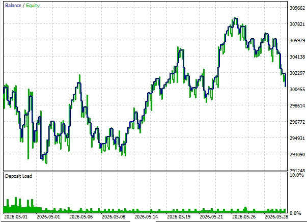
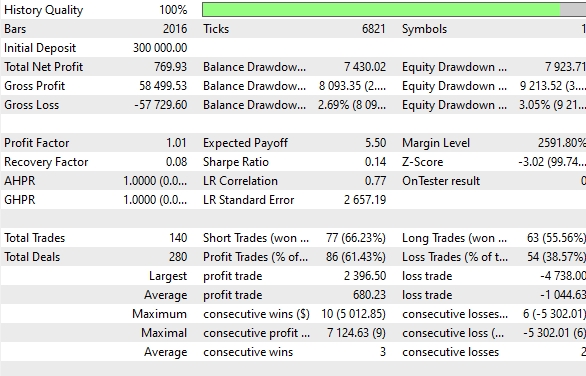
Let's look at a backtest of the Expert Advisor using opening prices and checking for new bars, for EURUSD H1 over the period May 1, 2026–June 1, 2026:
Final statistics:
In the first part, the problem of fixed weights was solved: 10,000 cells became live agents that are updated on every bar. In the second part, the problem of flat topology was solved: features and cells were converted into a graph structure. The third part addresses an even deeper problem: the fixed connection structure.
Now the feature graph learns on its own. It reinforces combinations that lead to profitable predictions and weakens combinations that lead to errors. This transforms the system from a set of indicators and rules into a self-organizing map of market cause-and-effect connections.
The practical implication is simple: a trader is no longer required to know in advance which combination of features will work tomorrow. The system automatically checks these combinations against the live data stream and reconfigures the internal graph without interrupting trading.
As a result, Cellular10K becomes a three-tier adaptive architecture:
- The trainable feature graph understands which market factors are currently connected;
- The graph of cellular automata transforms these connections into a collective decision made by 10,000 agents;
- The trading genome translates the trading decision into grid, risk, and position management parameters.
This is no longer just an Expert Advisor with a neural network. It is a market ecosystem in which features, agents, and trading parameters learn together.
| File name | File description |
|---|---|
| CellularNeuralNet10K.mqh | The CA 10K main module with a trainable feature graph and a graph of cellular automata |
| CellularBinaryPredictor10K.mqh | A binary predictor with a separate trainable feature graph over a 10-bar horizon |
| CA_Grid_10K.mq5 | An example of an Expert Advisor that combines CA, BPC, and adaptive trading genomes |
Translated from Russian by MetaQuotes Ltd.
Original article: https://www.mql5.com/ru/articles/23135
Warning: All rights to these materials are reserved by MetaQuotes Ltd. Copying or reprinting of these materials in whole or in part is prohibited.
This article was written by a user of the site and reflects their personal views. MetaQuotes Ltd is not responsible for the accuracy of the information presented, nor for any consequences resulting from the use of the solutions, strategies or recommendations described.