Neural Networks in Trading: A Spiking Architecture for Spatio-Temporal Market Analysis (Encoder)
 103
 0

Introduction
The market has never stood still. It has always moved to the rhythm of short bursts of activity, lulls, and unexpected reversals. For an experienced practitioner, this scenario has long been a familiar one. A price chart resembles the pulse of a living organism, and the tick stream is a series of barely perceptible signals that appear, disappear, and reappear, creating a complex web of market dynamics. And the more closely we examine these subtle shifts, the clearer it becomes that traditional data processing methods are not always fast enough to keep up with the pace of change in today's market.
Today, the market is moving faster than ever. Information spreads instantly. The algorithms respond with virtually no delay. And the tick stream has become so sparse yet information-rich that it is increasingly difficult to identify stable patterns within it. Traditional neural network architectures, which rely on dense data samples and fixed sampling rates, are beginning to fall short of real-time requirements. They require more memory, more computation, and more averaging, and therefore lose sight of the very essence of what is happening at the micro-event level.
This is where the concept of event-driven data processing originates. It brings us back to a fundamental principle: do not react to everything, but only to signals. If the market speaks, the model must listen. If the market falls silent, the model must remain calm. This approach is closer to the classical concepts of rational observation. We pay attention to the words, not the silence between them.
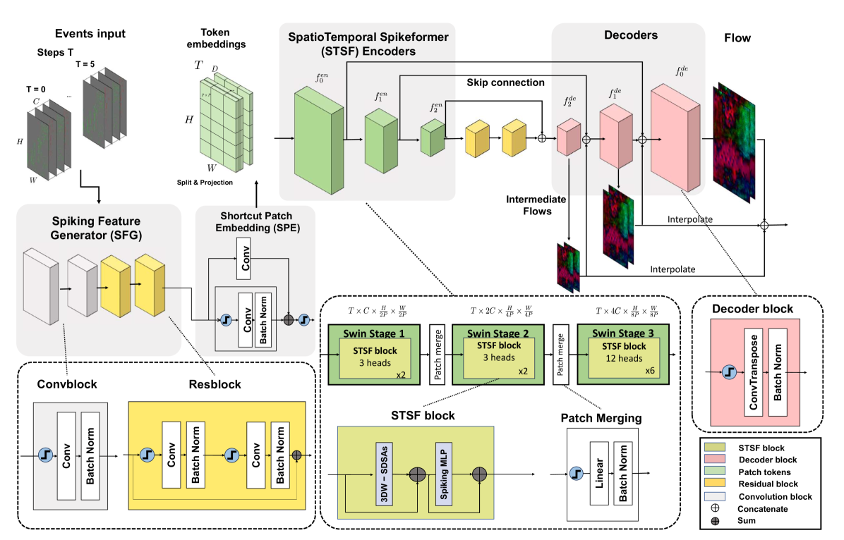
This is the principle behind the SDformerFlow framework, proposed in the research paper "SDformerFlow: Spatiotemporal swin spikeformer for event-based optical flow estimation". Its architecture is built around an event-based data representation — sparse but precise. It is designed for streams where every change has meaning. Where there is no regular time grid, but rather a sequence of pulses. Where the density of information changes from moment to moment. It is precisely this type of data that increasingly resembles the structure of a real market data stream.
SDformerFlow brings together several powerful ideas. First, it uses spiking neural networks, which are naturally well-suited to processing sparse sequences. A spiking neuron responds only when there is something for it to respond to — and this is important when working with financial data, where most ticks do not reflect a significant market move. Second, the architecture is based on transformers with sliding 3D windows, allowing it to examine dynamics in three dimensions at once: local space, temporal context, and their interactions. This classic multilayer approach makes the model flexible and highly scalable. Local detail captures micro-impulses, while broader patterns emerge at higher levels.
The third advantage is its hierarchical processing structure. In SDformerFlow, information is gradually aggregated and condensed through several levels of Spiking Patch Merge, while the time axis remains intact. This has a significant effect. The model can process short time intervals without losing synchronization. This is uncommon in time series analysis. Most architectures sacrifice temporal accuracy for the sake of abstraction; here, however, it is possible to preserve both.
For a financial markets professional, this structure is particularly valuable. It resembles the long-standing tradition of chart analysis. We start with minute-by-minute fluctuations, then look at the broader picture over the course of an hour, a day, or a week. SDformerFlow does something similar, but in the world of event data. It constructs signals while preserving context at every level. And if a spike in activity suddenly occurs in the tick stream, the model detects it both at the low level and within the structure of larger patterns.
Another important quality is energy and computational efficiency. Spiking architectures do not waste resources processing empty regions. This is especially important for financial data: the terms online learning and stream processing are not just buzzwords. They describe a real need. For traders and trading system developers, it is important that the model be lightweight, fast, and run reliably in the trading terminal. SDformerFlow, by its very nature, solves this problem elegantly. It works where dense architectures start to slow down.
It is precisely these features that make SDformerFlow an interesting tool for the financial markets. The model does not just analyze the price — it hears its rhythm. It takes into account the structure of events, not just averaged candlesticks. It detects local spikes and can distinguish noise from price movement. This approach is particularly consistent with the classical principles of technical analysis. We look for key points and market reactions; we don't calculate continuous functions.
The author's visualization of the SDformerFlow framework is shown below.
We aim to implement the proposed architecture using MQL5 and OpenCL, adapting it to the specific requirements of trading. The first phase has already been completed. We analyzed the basic components and laid the groundwork for the future implementation. Now it's time to move on and dive into building the model's key modules. A long and careful exploration of the SDformerFlow architecture lies ahead. And every new detail will bring us closer to creating an effective, rationally designed, and readily explainable tool for market analysis.
Attention Module
Now that we have reviewed the key benefits of the SDformerFlow framework, it is time to move from general concepts to practical implementation. Today's focus is on building the STSF encoder, one of the fundamental components of the entire model. Essentially, it is the workhorse of the framework. This is the component that transforms a sparse stream of events into a structured representation ready for further analysis.
The authors propose building an STSF encoder based on three key spiking elements:
- multi-head attention in event-based form;
- spiking MLP;
- a compact Patch-Merging block that neatly reduces the dimensionality.
This combination looks conventional at first glance — but only until we take a closer look. Here, each module operates on a specific principle. Reactions occur exclusively at moments of significant change. This makes processing rich in information yet computationally lightweight.
The logic behind the design of the STSF encoder resembles the work of a craftsperson who, layer by layer, removes the excess and leaves only the most expressive details. Multi-head spiking attention acts as a fine filter. It maintains a local focus, identifies relationships between events, and passes on only what truly affects the dynamics of the stream. A spiking MLP acts as a precise converter, adapting the feature structure for subsequent analysis while keeping the model lightweight. The block ends with Patch-Merging — the equivalent of a classic lens that gently compresses the space without disrupting the temporal structure of the sequence.
It is worth noting that the framework's authors have left us with an important architectural choice by offering two options for the event-driven attention module. The first option is closer to the classical school of transformers and relies on the dot-product mechanism — a precise, time-tested approach. It ensures a high level of model expressiveness, clear relationships between elements in the sequence, and stable behavior even with complex data.
The second option is a lightweight version of attention based on the QK line attention principle. Here, the computations are organized so that computational cost scales linearly with the length of the window being analyzed, rather than quadratically as in classical dot-product attention. This approach offers a noticeable advantage in long, event-rich streams, where even a small reduction in the computational load translates into a significant speed boost. And although linear attention is less resource-intensive, it retains the ability to identify key relationships in the data. This makes it particularly attractive for real-world trading streams, where the volume of events being analyzed can change several times per second.
As part of our work, we made a well-considered and entirely pragmatic decision to use the second option — linear QK-attention. It better aligns with the nature of event streams and allows for high processing speeds without noticeably compromising its ability to capture dependencies. For market data, this reduction in computational load plays a key role. For long sequences, the model must respond as quickly as the price changes.
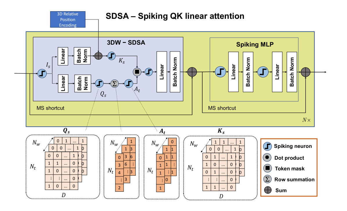
However, we did not limit ourselves to simply implementing the basic version. Linear attention opens up opportunities for further optimizations, especially in MQL5 and OpenCL environments. We will discuss the changes to the algorithm as we implement it.
Before we move on to constructing a new object and assembling complete linear attention blocks, we need to carry out a small but important preparatory task. Just as in traditional engineering practice, building a complex mechanism begins with debugging basic operations. In our case, we are talking about one of the fundamental operations on which a significant portion of the arithmetic in linear QK-attention is based — scalar-vector multiplication.
At first glance, this is an extremely simple operation — almost trivial. However, in an event-driven architecture, where computations are performed in streaming mode, it is used so frequently that even the slightest optimization noticeably increases the encoder's overall processing speed. That is precisely why we move it to the OpenCL context level and implement it as a separate, high-performance kernel. This approach reduces the load on the model's central logic and offloads routine computations to the GPU, where they can be naturally parallelized.
To do this, we create a compact yet efficient ScalarToVector kernel that performs element-wise multiplication of the input vector by a scalar.
__kernel void ScalarToVector(__global const float* scalar,
                             __global const float* vector_in,
                             __global float* vector_out
                            )
  {
   const size_t vec = get_global_id(0);
   const size_t d  = get_global_id(1);
   const size_t vectors = get_global_size(0);
   const size_t dimension = get_global_size(1);
//---
   float sc = IsNaNOrInf(scalar[vec], 0.0f);
   int shift = RCtoFlat(vec, d, vectors, dimension, 0);
   float v = IsNaNOrInf(vector_in[shift], 0.0f);
//---
   vector_out[shift] = IsNaNOrInf(sc * v, 0.0f);
  }
The structure is clear and strictly linear. Each work-item processes its own pair of indices, retrieves the scalar value, handles potentially invalid input data using IsNaNOrInf, multiplies the scalar by the corresponding vector element, and writes the result to the output buffer.
This function will serve as a building block for future computational chains. It will allow us to quickly scale operations on feature vectors.
Along with the forward pass, we need to implement the error backpropagation mechanism right away. In trainable models, every operation must have a backward counterpart that allows gradients to be correctly propagated to the preceding layers. This is especially important for linear attention, where even simple operations are part of long computation chains. Failing to compute gradients at such an early stage means leaving a gap that will later result in incorrect weight updates and a loss of convergence.
The backpropagation algorithm in the ScalarToVectorGrad kernel is surprisingly simple and, at the same time, elegant. It is like a good old-fashioned clock mechanism, where every cog works toward the common goal.
__kernel void ScalarToVectorGrad(__global const float* scalar,
                                 __global float* scalar_gr,
                                 __global const float* vector_in,
                                 __global float* vector_in_gr,
                                 __global float* vector_out_gr,
                                 const int dimension
                                )
  {
   const size_t vec = get_global_id(0);
   const size_t loc  = get_local_id(1);
   const size_t vectors = get_global_size(0);
   const size_t total_loc = get_local_size(1);
//---
   __local float temp[LOCAL_ARRAY_SIZE];
At the very beginning, each thread determines its own scope of work: the vector's index in the batch, the thread's position within the work-group, and the number of threads that collectively process the same vector. This sets the pace for the entire computation, allowing the load to be distributed evenly.
To avoid repeatedly accessing global memory, one thread preloads the scalar into a temporary local buffer. The synchronization barrier forces the other threads to wait a moment until the value is in place, after which each participant gains quick access to it, just as if it were a shared reference book lying in the middle of the table.
   if(loc == 0)
      temp[0] = IsNaNOrInf(scalar[vec], 0.0f);
   BarrierLoc
   float sc = temp[0];
   float sc_gr = 0;
Next comes the main work: each thread handles several vector coordinates assigned according to its index within the group, iterating through them step by step to the end of the vector. This ensures massive parallelism, where each thread is responsible for its own part of the computation.
   for(int d = loc; d < dimension; d += total_loc)
     {
      int shift = RCtoFlat(vec, d, vectors, dimension, 0);
      float v = IsNaNOrInf(vector_in[shift], 0.0f);
      float grad = IsNaNOrInf(vector_out_gr[shift], 0.0f);
      vector_in_gr[shift] = IsNaNOrInf(grad * sc, 0.0f);
      sc_gr += IsNaNOrInf(v * grad, 0.0f);
     }
At each of these steps, three key actions take place. First, the thread retrieves the next vector element from the input array, along with the gradient of the output value. It then immediately computes the gradient with respect to the input element itself by simply multiplying the output gradient by the stored scalar. Finally, in parallel with this, the thread begins accumulating its contribution to the gradient with respect to the scalar. This contribution is always simple: the product of the input value and the output gradient. As a result, each thread produces a small portion of the total sum.
Once the group members have finished iterating over their elements, it is time to combine the accumulated results. The entire work-group uses a simple reduction procedure: each thread places its partial sum into a local buffer, and then the values are added together in the standard way until a single final value remains. It is equally accessible to all threads, but only one thread — the one responsible for writing the final gradient with respect to the scalar for the current vector — should write it to the global array.
   sc_gr = LocalSum(sc_gr, 1, temp);
   if(loc == 0)
      scalar_gr[vec] = sc_gr;
  }
The kernel then finishes execution smoothly, leaving behind two neatly filled arrays. The first contains the gradients with respect to the input vector, computed elementwise and stored at the same indices as the original data. The second is the gradient with respect to the scalar, computed through the combined work of all threads in the work-group. The entire procedure runs smoothly, predictably, and efficiently, ensuring correct error backpropagation for scalar-vector multiplication and making it suitable for large-scale neural network computations within future STSF encoder modules.
Here, we are entering a new, more significant phase of implementation. After a small but essential amount of preparatory work in the OpenCL program, we can build the first fully fledged computational module — the CNeuronSpikeQKAttention object. The structure looks massive and multi-layered, but inside it follows a strict logic, like a well-designed machine where every part has its own specific function.
class CNeuronSpikeQKAttention :  public CNeuronBaseOCL
  {
protected:
   CNeuronSpikeConvBlock      cQK;
   CNeuronSpikeActivation     cSpikeQK;
   CNeuronBaseOCL             cQ;
   CNeuronBaseOCL             cK;
   CNeuronMultiWindowsConvOCL cScore;
   CNeuronSpikeActivation     cSpikeScore;
   CLayer                     cProject;
   //---
   virtual bool      feedForward(CNeuronBaseOCL *NeuronOCL) override;
   virtual bool      updateInputWeights(CNeuronBaseOCL *NeuronOCL) override;
   virtual bool      calcInputGradients(CNeuronBaseOCL *NeuronOCL) override;

public:
                     CNeuronSpikeQKAttention(void) {};
                    ~CNeuronSpikeQKAttention(void) {};
   //---
   virtual bool      Init(uint numOutputs, uint myIndex, COpenCLMy *open_cl,
                          uint units, uint window, uint heads, uint dimension_k,
                          ENUM_OPTIMIZATION optimization_type, uint batch);
   //---
   virtual int       Type(void) override const  {  return defNeuronSpikeQKAttention;   }
   //--- methods for working with files
   virtual bool      Save(int const file_handle) override;
   virtual bool      Load(int const file_handle) override;
   //---
   virtual void      SetOpenCL(COpenCLMy *obj)   override;
   //---
   virtual bool      WeightsUpdate(CNeuronBaseOCL *source, float tau) override;
   virtual void      SetActivationFunction(ENUM_ACTIVATION value) override { };
   virtual void      TrainMode(bool flag) override;
   virtual bool      Clear(void) override;
  };
The class structure shown here declares a number of auxiliary components. The cQK and cSpikeQK pair is responsible for generating preliminary spiking representations for queries and keys, creating the dense, efficient encoding that makes the entire framework unique.
Next come two basic objects — cQ and cK — which essentially represent separate channels for generating Q and K. Next comes the cScore block, which uses multi-channel convolution to produce a matrix of attention logits. The cSpikeScore block supplements these calculations with spiking activation, helping to produce a more expressive, energy-efficient response. The cProject module completes the chain by bringing the results together and generating the final multidimensional representation.
The initialization method carefully constructs the internal geometry of the entire object and ensures that every component is ready for use within the OpenCL context.
bool CNeuronSpikeQKAttention::Init(uint numOutputs, uint myIndex, COpenCLMy *open_cl,
                                   uint units, uint window, uint heads, uint dimension_k,
                                   ENUM_OPTIMIZATION optimization_type, uint batch)
  {
   if(!CNeuronBaseOCL::Init(numOutputs, myIndex, open_cl, window * units, optimization_type, batch))
      return false;
   activation = None;
First, the parent class's initialization method is called. Here, the neuron's main resources are created, taking into account the total number of results and a pointer to the OpenCL context. If the base initialization fails, the method immediately returns false, protecting the system from an invalid state.
Next, the internal blocks are initialized in stages. The cQK block is the heart of the QK attention mechanism, where the kernels for generating Q and K are created. We pass the window size, the number of neurons, and the sizes along the key dimensions.
   uint index = 0;
   if(!cQK.Init(0, index, OpenCL, window, window, dimension_k * heads * 2, units, 1, optimization, iBatch))
      return false;
   index++;
   if(!cSpikeQK.Init(0, index, OpenCL, cQK.Neurons(), optimization, iBatch))
      return false;
Next, a layer is created to transform the signals from the QK block into spiking activity.
The cQ and cK objects each receive half of the neurons from QK, which makes sense given the split into Q and K. We also assign them an activation function synchronized with cSpikeQK.
   index++;
   if(!cQ.Init(0, index, OpenCL, cQK.Neurons() / 2, optimization, iBatch))
      return false;
   cQ.SetActivationFunction((ENUM_ACTIVATION)cSpikeQK.Activation());
   index++;
   if(!cK.Init(0, index, OpenCL, cQ.Neurons(), optimization, iBatch))
      return false;
   cK.SetActivationFunction((ENUM_ACTIVATION)cSpikeQK.Activation());
Next, an array of windows is created according to the specified number of attention heads, and the attention computation block is initialized.
   index++;
   uint windows[];
   if(ArrayResize(windows, heads) < (int)heads)
      return false;
   ArrayFill(windows, 0, heads, dimension_k);
   if(!cScore.Init(0, index, OpenCL, windows, 1, units, 1, optimization, iBatch))
      return false;
   cScore.SetActivationFunction(None);
Each attention head is assigned its own window of dimension dimension_k.
It is worth noting that in the original version of the SDformerFlow framework, the authors simply sum the elements of the query vector (Query) when calculating the score. We took it a step further and implemented weighted summation with trainable coefficients, which allows each component of the vector to make its own individual contribution to the final value.
In addition, integrating the multi-window convolution object makes it possible to train separate parameters for each attention head. This opens up opportunities for more flexible and adaptive model configuration. Each attention head can account for different characteristics of the signal and develop its own combinations of weights. As a result, the algorithm becomes more sensitive to the data structure and more accurate in its predictions, while maintaining overall compactness and computational efficiency.
The next step is to create a spiking layer for scoring. It converts the results into spikes that define masks for the key tensor.
   index++;
   if(!cSpikeScore.Init(0, index, OpenCL, cScore.Neurons(), optimization, iBatch))
      return false;
Next, the projection block is prepared: it is cleared and granted access to OpenCL.
   cProject.Clear();
   cProject.SetOpenCL(OpenCL);
The first object in the projection module is the base neural layer, in which we will store the results of multiplying the key tensor by the attention mask.
   index++;
   CNeuronBaseOCL* neuron = new CNeuronBaseOCL();
   if(!neuron ||
      !neuron.Init(0, index, OpenCL, cK.Neurons(), optimization, iBatch) ||
      !cProject.Add(neuron))
     {
      DeleteObj(neuron)
      return false;
     }
We carefully check every step. If something goes wrong, the object is deleted to prevent memory leaks.
The method concludes with the initialization of the convolutional block.
   index++;
   CNeuronSpikeConvBlock* conv = new CNeuronSpikeConvBlock();
   if(!conv ||
      !conv.Init(0, index, OpenCL, dimension_k * heads, dimension_k * heads,
                                  window, units, 1, optimization, iBatch) ||
      !cProject.Add(conv))
     {
      DeleteObj(conv)
      return false;
     }
//---
   return true;
  }
This block aggregates signals by combining all attention heads into a single structure.
After successfully adding all components, the method returns true, indicating that the object is fully ready.
As a result, the initialization method carefully constructs a coherent, multilevel attention structure based on spiking neurons. Each block is initialized according to a strict geometric layout, the activation functions are synchronized, and error checking at every step ensures stability. This sequence of steps transforms a potentially chaotic set of components into an organized, flexible architecture that is ready for training and processing streaming data.
The feedForward method is responsible for processing the input data stream step by step and converting it into a neatly organized structure of attention signals. Unlike the standard implementation of the framework, where the elements of the query vector are simply summed, we use weighted summation with trainable coefficients, which allows each component of the Q vector to make an individual contribution. This gives the algorithm the flexibility and precision to adapt to the characteristics of the input signal.
bool CNeuronSpikeQKAttention::feedForward(CNeuronBaseOCL *NeuronOCL)
  {
   if(!cQK.FeedForward(NeuronOCL))
      return false;
First, the signal under analysis is fed into the QK block, which forms kernels for generating the Q and K vectors, laying the foundation for attention.
The signal is then converted into spiking activity using cSpikeQK.
   uint units = cQK.GetUnits();
   uint window = cQK.GetWindow();
   uint dimension_k = cScore.GetWindow(0);
   uint hd = cQK.GetFilters() / 2;
   uint heads = hd / dimension_k;
//---
   if(!cSpikeQK.FeedForward(cQK.AsObject()))
      return false;
   if(!DeConcat(cQ.getOutput(), cK.getOutput(), cSpikeQK.getOutput(), hd, hd, units))
      return false;
After that, the combined output is split into separate Query and Key entities. This step ensures that the data for each attention head is precisely aligned, guaranteeing signal consistency at all levels.
The next step is to compute the scores. The vector Q passes through the multi-window convolutional block cScore, where weighted summation is performed using individual parameters for each attention head.
   if(!cScore.FeedForward(cQ.AsObject()))
      return false;
   if(!cSpikeScore.FeedForward(cScore.AsObject()))
      return false;
Each attention head can adapt to distinct characteristics of the stream being analyzed, making the model sensitive to local data structures.
The scoring results are then converted into spikes using cSpikeScore.
After that, the scalar scores are multiplied by the K vectors, producing a consistent output for each attention head.
   CNeuronBaseOCL* neuron = cProject[0];
   if(!neuron ||
      !ScalarToVector(cSpikeScore.getOutput(), cK.getOutput(), neuron.getOutput(), dimension_k))
      return false;
Next, each neuron in the projection block processes the signal from the previous one, creating a chain of transformations that carefully aggregate the data stream and form the final result tensor.
   for(int i = 1; i < cProject.Total(); i++)
     {
      neuron = cProject[i];
      if(!neuron ||
         !neuron.FeedForward(cProject[i - 1]))
         return false;
     }
The final step is to add the residual connections. The outputs of the projection block are added to the input data.
   if(!SumAndNormilize(NeuronOCL.getOutput(), neuron.getOutput(), Output, window, false, 0, 0, 0, 1))
      return false;
//---
   return true;
  }
Thus, our forward pass method creates an adaptive, learnable attention mechanism. Each attention head has its own parameters, and the query vector is formed taking into account the individual influence of each element. This makes the algorithm more accurate and sensitive to the characteristics of time series, which is particularly important for processing highly dynamic financial streams with unpredictable structures.
The calcInputGradients method is responsible for backpropagating the error through all components of the object. Its task is to accurately compute the gradients for each element and prepare the network for weight adjustment, ensuring that the model is trained accurately.
bool CNeuronSpikeQKAttention::calcInputGradients(CNeuronBaseOCL *NeuronOCL)
  {
   if(!NeuronOCL)
      return false;
//---
   uint units = cQK.GetUnits();
   uint window = cQK.GetWindow();
   uint dimension_k = cScore.GetWindow(0);
   uint hd = cQK.GetFilters() / 2;
   uint heads = hd / dimension_k;
First, the method checks the validity of the received pointer to the input neuron object. If the object is missing, further calculations are not possible. This is a basic safeguard that ensures stability.
Next, the structure's parameters are retrieved. They are needed to ensure that the dimensions of the signals and gradients match exactly at all levels of the model.
The next step is to work with the projection block (cProject). Here, the error gradient received from downstream model objects is adjusted using the derivative of the activation function of the final projection layer.
   CNeuronBaseOCL* neuron = cProject[-1];
   if(!neuron ||
      !DeActivation(neuron.getOutput(), neuron.getGradient(), Gradient, neuron.Activation()))
      return false;
This restores the correct gradients, which will be used to calculate the errors in the previous layers.
Next, starting with the second-to-last neuron, backpropagation of the error is performed across all layers of the projection.
   for(int i = cProject.Total() - 2; i >= 0; i--)
     {
      neuron = cProject[i];
      if(!neuron ||
         !neuron.CalcHiddenGradients(cProject[i + 1]))
         return false;
     }
Each neuron receives gradients from the next layer, forming a chain of correct signal adjustments from output to input.
Next, we split the gradients between the scoring block and the vector space of the K block.
   if(!ScalarToVectorGrad(cSpikeScore.getOutput(), cSpikeScore.getGradient(),
                          cK.getOutput(), cK.getGradient(),
                          neuron.getGradient(), dimension_k))
      return false;
The method carefully distributes the error to the scoring block and individual neurons of the K block, taking into account the weighted parameters we used in feedForward. This is a key point for adaptive learning. Each attention head receives individual gradient signals.
The next steps are backpropagation through the Q and Score blocks.
   if(!cScore.CalcHiddenGradients(cSpikeScore.AsObject()))
      return false;
   if(!cQ.CalcHiddenGradients(cScore.AsObject()))
      return false;
The Q block and the multi-window convolution receive gradients, allowing the convolution parameters of each attention head to be trained. This ensures the model's adaptability and accuracy when working with various data structures.
The gradients from Q and K are then merged back into the spiking QK block.
   if(!Concat(cQ.getGradient(), cK.getGradient(), cSpikeQK.getGradient(), hd, hd, units))
      return false;
   if(!cQK.CalcHiddenGradients(cSpikeQK.AsObject()))
      return false;
This is the step where all the computed gradients are consolidated and passed to the main QK block, ensuring that all parameters are updated in a coordinated manner.
The error then propagates to the input data level.
   if(!NeuronOCL.CalcHiddenGradients(cQK.AsObject()))
      return false;
   neuron = cProject[-1];
   if(!DeActivation(NeuronOCL.getOutput(), neuron.getPrevOutput(), Gradient, NeuronOCL.Activation()))
      return false;
   if(!SumAndNormilize(NeuronOCL.getGradient(), neuron.getPrevOutput(), NeuronOCL.getGradient(), window,
                                                                                     false, 0, 0, 0, 1))
      return false;
//---
   return true;
  }
Here, the external object receives the correct gradients via two information streams, including the residual connection pathway, with the characteristics of its activation function taken into account.
As a result, the calcInputGradients method provides a complete backpropagation mechanism in which each component correctly receives and distributes gradients.
STSF block
Having completed the attention module, the natural next step is to integrate the next component of the STSF block — a spiking MLP with residual connections. Upon closer inspection, its architecture is identical to that of the MSRes block that we implemented earlier. This gives us a unique advantage: both key elements — the spiking attention block and the multilayer residual network — already exist in the code, and now they can be combined into a single, cohesive structure.
The CNeuronSDSA class inherits the functionality of the MSRes block, extending it with spiking attention.
class CNeuronSDSA :  public CNeuronMSRes
  {
protected:
   CNeuronSpikeQKAttention cAttention;
   //---
   virtual bool      feedForward(CNeuronBaseOCL *NeuronOCL) override;
   virtual bool      updateInputWeights(CNeuronBaseOCL *NeuronOCL) override;
   virtual bool      calcInputGradients(CNeuronBaseOCL *NeuronOCL) override;

public:
                     CNeuronSDSA(void) {};
                    ~CNeuronSDSA(void) {};
   //---
   virtual bool      Init(uint numOutputs, uint myIndex, COpenCLMy *open_cl,
                          uint units, uint window, uint heads, uint dimension_k,
                          ENUM_OPTIMIZATION optimization_type, uint batch);
   //---
   virtual int       Type(void) override const  {  return defNeuronSDSA;   }
   //--- methods for working with files
   virtual bool      Save(int const file_handle) override;
   virtual bool      Load(int const file_handle) override;
   //---
   virtual void      SetOpenCL(COpenCLMy *obj)   override;
   //---
   virtual bool      WeightsUpdate(CNeuronBaseOCL *source, float tau) override;
   virtual void      TrainMode(bool flag) override;
   virtual bool      Clear(void) override;
  };
A key component within it is the cAttention object (CNeuronSpikeQKAttention), which implements spiking QK attention with multi-window convolution and weighted summation, as described above. It is this object that makes the SDSA block adaptive to the structure of the analyzed stream, allowing each attention head to learn its own parameters and generate individual gradients.
All components of the block are initialized in the concise Init method. It carefully constructs the object's architecture and ensures that each element is ready to process streaming data.
bool CNeuronSDSA::Init(uint numOutputs, uint myIndex, COpenCLMy *open_cl,
                       uint units, uint window, uint heads, uint dimension_k,
                       ENUM_OPTIMIZATION optimization_type, uint batch)
  {
   if(!CNeuronMSRes::Init(numOutputs, myIndex, open_cl, units, window, 1, optimization_type, batch))
      return false;
First, the parent MSRes block is initialized. This is where the main residual layers of the MLP are created. The MSRes block forms the fundamental structure of the object, enabling efficient signal aggregation and preserving residual connections that maintain the stability of the gradients. If the base initialization fails, the method immediately returns false, preventing further errors.
The next step is to initialize the spiking attention block.
   if(!cAttention.Init(0, 0, OpenCL, units, window, heads, dimension_k, optimization, iBatch))
      return false;
//---
   return true;
  }
The cAttention block implements QK attention using multi-window convolution and weighted summation for each head.
After both components have been successfully initialized, the method returns true, indicating that CNeuronSDSA is fully ready for operation. The block combines the stability of MSRes with the adaptability of spiking attention, creating a unified mechanism capable of simultaneously identifying local and global dependencies in the data.
The forward pass algorithm is implemented in the feedForward method. Everything here is structured in an extremely concise and linear manner.
bool CNeuronSDSA::feedForward(CNeuronBaseOCL *NeuronOCL)
  {
   if(!cAttention.FeedForward(NeuronOCL))
      return false;
   return CNeuronMSRes::feedForward(cAttention.AsObject());
  }
First, the signal under analysis is processed by the spiking QK attention object. Its output is then fed into an MLP with residual connections, whose functionality is provided by mechanisms inherited from the parent class.
This linearity is possible because the residual connection mechanisms are already built into each component of the block. As a result, the forward pass becomes predictable, transparent, and easy to analyze, which greatly simplifies understanding of how the block works and reduces the likelihood of errors when integrating it into larger architectures.
Backpropagation methods are structured similarly: they follow the same logic, carefully propagating gradients through the attention mechanism and the MLP. To keep the text from becoming too dense, we leave these for you to explore on your own; the complete code for the CNeuronSDSA class, including the implementation of all methods, is provided in the attachment.
Thus, CNeuronSDSA demonstrates an ideal combination of adaptability and structural clarity. Complex attention operations and multi-layer processing are integrated into a compact, easy-to-read sequence, making the block particularly well-suited for building complex STSF structures and processing streaming data.
We've done a lot of work today and deserve a short break to let it all sink in. In the next article, we will continue our step-by-step approach and bring it to its logical conclusion, revealing all the remaining details and consolidating the results we have achieved.
Conclusion
We examined in detail the design and integration of a spiking attention block with a residual MLP architecture within the STSF block. We demonstrated how using weighted summation of Query and multi-window convolution for each attention head improves the algorithm's adaptability and the accuracy of streaming data processing. The CNeuronSDSA implementation combines the stability of the MSRes block with the flexibility of spiking attention, creating a unified mechanism capable of identifying local and global dependencies.
In the next article, we will continue our work by focusing on testing, performance evaluation, and the practical application of the approaches we have implemented, which will allow us to fully realize the potential of the SDformerFlow framework.
Links
- SDformerFlow: Spatiotemporal swin spikeformer for event-based optical flow estimation
- Other articles in this series
Software used in this article
| # | Name | Type | Description |
|---|---|---|---|
| 1 | Study.mq5 | Expert Advisor | Expert Advisor for offline model training |
| 2 | StudyOnline.mq5 | Expert Advisor | Expert Advisor for online learning of models |
| 3 | Test.mq5 | Expert Advisor | Model testing Expert Advisor |
| 4 | Trajectory.mqh | Class library | Structure describing the system state and model architectures |
| 5 | NeuroNet.mqh | Class library | Class library for building a neural network |
| 6 | NeuroNet.cl | Library | Code library for an OpenCL program |
Translated from Russian by MetaQuotes Ltd.
Original article: https://www.mql5.com/ru/articles/20377
Warning: All rights to these materials are reserved by MetaQuotes Ltd. Copying or reprinting of these materials in whole or in part is prohibited.
This article was written by a user of the site and reflects their personal views. MetaQuotes Ltd is not responsible for the accuracy of the information presented, nor for any consequences resulting from the use of the solutions, strategies or recommendations described.