

L-Moments for Robust Return Profiling in MQL5: A Distribution-Shape Regime Validator
 22
 0

Introduction
Skewness and kurtosis are two of the most common shape statistics quoted in trading literature, and both are quietly fragile. They are built from cubed and fourth-power deviations from the mean, which means a single 6-sigma bar in a rolling window can dominate the whole estimate. On a return series that occasionally contains flash-crash bars, broker requotes, or thin-liquidity gaps, this is not a corner case – it is a routine occurrence, and it means a classical kurtosis reading can swing wildly for reasons that have nothing to do with the underlying regime.
L-moments are an alternative moment system built from linear combinations of order statistics – the sorted sample itself – rather than powers of deviations. Because sorting and linear weighting cannot blow up the way cubing and raising to the fourth power can, L-moment shape ratios stay bounded and numerically well-behaved even when a handful of outliers sit in the window – not immune to them, but far less easily swayed by them than an estimator that cubes or raises deviations to the fourth power.
This article builds a native MQL5 pipeline to compute L-moments from real probability-weighted moments. It then tests them in a rolling walk-forward validator against the conventional Pearson estimators they are proposed as an alternative to, across three real pair/timeframe cases. In two of those three cases, the classical estimator achieved a higher F1 score. The numerical case for L-moments holds regardless of that result, for reasons the Math section makes precise; whether that numerical advantage also means a better trading signal is a separate, empirical question this article tests rather than assumes.
L-moments themselves are not new; Hosking introduced them in 1990, and they have been standard practice in hydrology and extreme-value statistics for decades, precisely because rainfall and flood records share the same fat-tailed, outlier-prone character that FX and index returns do. What follows adapts that estimator to MQL5 from first principles – no external statistics library, no ALGLIB, nothing but native arrays and the formulas themselves – and then puts it through a real, data-first walk-forward test rather than a purely theoretical treatment.
Scope. This project is a diagnostic script, not an Expert Advisor. It walks forward through real historical bars once, using CopyRates() and iATR(), and prints a precision/recall verdict for each flag type. No Strategy Tester run is involved anywhere in this article.
Contents
- The Math: From PWMs to L-Moment Ratios
- Architecture
- LMomentsCore.mqh: The PWM-to-L-Moment Pipeline
- ReturnWindowStats.mqh: The Rolling Window and the Conventional Baseline
- LMoment_RegimeValidator.mq5: The Walk-Forward Script
- Testing
- Limitations and Practical Considerations
- Conclusion
The Math: From PWMs to L-Moment Ratios
L-moments are derived in two stages. The first stage is the probability-weighted moment (PWM), a linear functional of the sorted sample that never squares or cubes anything:
// unbiased sample PWM of order k, for a sample sorted ascending
// x(1) <= x(2) <= ... <= x(n), 1-indexed

b_k = (1/n) * sum_{i=1}^{n} [ (i-1)(i-2)...(i-k) / (n-1)(n-2)...(n-k) ] * x(i)
b0 is just the sample mean – the product in the numerator is empty (equals 1) when k=0. Each higher order progressively down-weights the low-ranked observations, which is what lets b1..b3 carry shape information without ever raising a deviation to a power. That is the source of L-moments' resistance to outliers: a single extreme value contributes to this formula only in proportion to its own weight, linearly, never raised to a power the way a cubed or fourth-power deviation is – so its influence grows additively with the value's rank-based weight, not exponentially with its size. That makes a large outlier harder to dominate the estimate with, not impossible to; the worked example below puts a real number on exactly how much harder.
The second stage folds the four PWMs into the first four L-moments via Hosking's (1990) linear map:
lambda1 = b0
lambda2 = 2*b1 - b0
lambda3 = 6*b2 - 6*b1 + b0
lambda4 = 20*b3 - 30*b2 + 12*b1 - b0
lambda1 is a location measure (equal to the mean). lambda2 (L-scale) is well-defined for any window of 4 or more points, because it is a linear combination with no division anywhere in it. By contrast, tau3 and tau4 both divide by lambda2 and are undefined when lambda2 is zero. The implementation in the next section still signals failure for the whole Compute() call when lambda2 is numerically zero, because that call's contract is to hand back usable tau3/tau4 alongside it, not lambda2 in isolation – lambda1 through lambda4 are set to their correctly computed values either way, only tau3/tau4 are zeroed out. The two ratios this article actually tests are scale-free shape descriptors, directly analogous to skewness and kurtosis but built from the L-moments instead of central moments:
tau3 = lambda3 / lambda2     // L-skewness
tau4 = lambda4 / lambda2     // L-kurtosis
tau4 is the one this article's validator actually flags on: a spike in tau4 is read as a signal that the return distribution over the current window has developed heavier, more extreme tails than its own recent history – the L-moment analogue of "kurtosis just jumped," but computed from a formula that is structurally harder to distort with the very outliers it is trying to detect, since those outliers contribute linearly rather than through a cubed or fourth-power term.
A concrete worked example makes the difference tangible. Take a 60-return window – the same window length the validator itself uses – built from small, ordinary noise with two larger bars inserted (a spread spike and a news bar, roughly 0.85% and -0.71%, sitting inside 58 bars of typical sub-0.1% noise). Computing both estimators on this window, then again after replacing just those two bars with ordinary-sized noise, shows how differently each one reacts to the same two data points:
For readers who want to verify these numbers directly: the 60-value window is numpy.random.seed(7) followed by numpy.random.normal(0, 0.0006, 60), with index 15 set to 0.0085 and index 42 set to -0.0071 for the outlier case. The clean comparison re-seeds with numpy.random.seed(2270) and redraws those same two indices from the same distribution before recomputing both estimators.
// 60-bar window, two outlier bars included
tau4 = 0.4572          g2 (excess kurtosis) = 18.9243

// same window, those two bars replaced with typical-scale noise
tau4 = 0.1543          g2 (excess kurtosis) = -0.3616

// absolute swing caused by just 2 bars out of 60
tau4 swing = 0.30 (about 2x its clean-sample value)
g2   swing = 19.29 (about 53x its clean-sample value)
Two bars out of sixty – roughly 3% of the window – are enough to send the classical excess kurtosis from a mildly negative, unremarkable -0.36 up to 18.92, a swing of more than 19 full units with no natural ceiling. tau4 moves too (it is not claiming the two bars are irrelevant), but it moves from 0.15 to 0.46, entirely within the range a shape ratio built from sorted-order weights can actually reach. This is precisely the mechanism described earlier, made numeric rather than abstract: g2's cubed and fourth-power terms let two extreme values dominate a sum of sixty, while tau4's linear order-statistic weights cannot be dominated the same way.
Architecture
The pipeline is three files deep, and every step in it operates on the exact same rolling window of log returns – the robust and conventional estimators are never allowed to see different data, since that would make any comparison between them meaningless. CReturnWindowStats owns the window and hands out a sorted copy to CLMoments::Compute for the L-moment side, and computes the Pearson baseline itself on the same buffer. Both results feed a pair of CRollingBaseline instances that track each metric's own recent history, so a "spike" is always relative to what that specific metric has been doing lately on that specific instrument – not a hard-coded constant that would mean something different on EURUSD than on USDJPY.
L-Moment Regime Validator: Data Flow
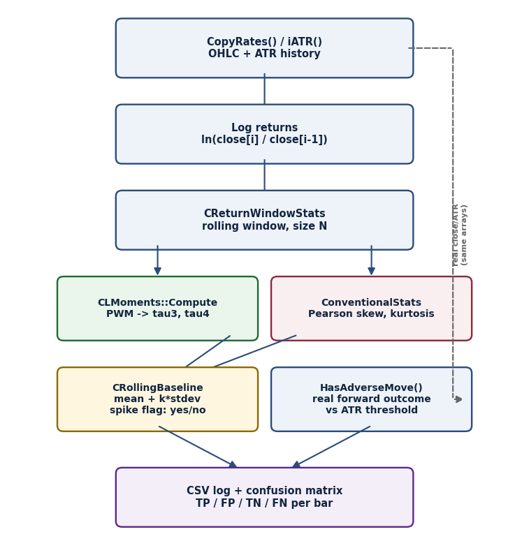
Fig. 1. CRollingBaseline and HasAdverseMove() are computed independently from separate inputs and only converge at the final confusion matrix.
The right-hand side of that diagram is the part that keeps the comparison honest: the forward outcome (HasAdverseMove()) is computed from real subsequent closes and a real ATR reading, and every flag is scored against it via a genuine confusion matrix – true/false positive, true/false negative – not a subjective read of a chart.
Two design choices in this architecture are worth calling out specifically. First, the two spike baselines (tau4's and conventional kurtosis's) are tracked by entirely separate CRollingBaseline instances rather than one shared object – a design that would be tempting to simplify, but the two metrics live on different numeric scales (tau4 is naturally bounded near [-1, 1]; excess kurtosis is not bounded at all, as the worked example above shows) and mixing their histories into one running mean/stdev would make the adaptive threshold meaningless for both. Second, this project is deliberately a script, not an Expert Advisor or indicator. It runs once and has no OnTick() state. This design allows a single-pass walk over all available history to compute a precision/recall verdict without using the Strategy Tester.
LMomentsCore.mqh: The PWM-to-L-Moment Pipeline
The class declaration is a single static utility – no per-instance state at all, since every call receives its own sorted array. Both methods are marked static for exactly that reason:
//+------------------------------------------------------------------+
//| CLMoments                                                        |
//| Stateless utility class: converts a pre-sorted sample of log     |
//| returns into unbiased Probability-Weighted Moments (PWMs) and    |
//| then into L-moments (lambda1..lambda4) and the two scale-free    |
//| L-moment ratios (L-skewness tau3, L-kurtosis tau4). All methods  |
//| are static – this class carries no per-instance state, so a      |
//| single sorted array is the only input any call needs.            |
//+------------------------------------------------------------------+
class CLMoments
  {
private:
   //--- probability-weighted moment of a given order (0..3), computed
   //--- directly from the sorted sample via the unbiased plotting-
   //--- position estimator (Hosking & Wallis, 1997)
   static double     ComputePWM(const double &sorted[],int order);

public:
   //--- full pipeline: sorted returns in, PWMs b0..b3 folded into
   //--- lambda1..lambda4, then tau3/tau4 derived as scale-free ratios
   static bool       Compute(const double &sorted_returns[],
                             double &lambda1,double &lambda2,
                             double &lambda3,double &lambda4,
                             double &tau3,double &tau4);
  };
ComputePWM – implements the PWM formula from the Math section directly, term by term. The denom_product is built once outside the sample loop since it does not depend on i, and the i-1 < order guard skips the leading terms whose numerator product would contain a zero factor – computing those explicitly would just waste cycles multiplying by zero every time.
//+------------------------------------------------------------------+
//| CLMoments::ComputePWM                                            |
//| Computes the order-th unbiased sample probability-weighted       |
//| moment b_order = (1/n) * sum_i w_i(order) * x_(i), where x_(i)   |
//| is the i-th smallest value (1-indexed) and w_i(order) is the     |
//| product of (i-1)(i-2)...(i-order) divided by the matching        |
//| product of (n-1)(n-2)...(n-order). order=0 reduces to the        |
//| plain sample mean; order>0 progressively down-weights the        |
//| lower order statistics, which is what lets b1..b3 carry shape    |
//| information without ever squaring or cubing a deviation –        |
//| the source of L-moments' robustness to a handful of outliers.    |
//+------------------------------------------------------------------+
static double CLMoments::ComputePWM(const double &sorted[],int order)
  {
   int n=ArraySize(sorted);
   if(n<=order)                                     // not enough points
      return(0.0);                                  // to form this order

   double numerator_product;                        // running (i-1)...(i-order)
   double denom_product=1.0;                        // running (n-1)...(n-order)
   for(int k=1; k<=order; k++)
      denom_product*=(n-k);                          // build once, reused per i

   double sum=0.0;
   for(int i=1; i<=n; i++)
     {
      if(i-1<order)                                 // product has a zero factor
         continue;                                  // for i<=order, skip early

      numerator_product=1.0;
      for(int k=1; k<=order; k++)
         numerator_product*=(i-k);

      sum+=(numerator_product/denom_product)*sorted[i-1];
     }
   return(sum/n);
  }
Compute – calls ComputePWM four times (orders 0 through 3), applies the Hosking linear map exactly as written in the Math section, and then divides to get the two ratios. The two early-return guards both matter for a live validator: n<4 catches a window that has not been sized correctly upstream, and the lambda2 near-zero check catches a window of near-constant returns (a dead or halted market), where tau3/tau4 would otherwise divide by a number close to zero and produce a nonsense spike.
//+------------------------------------------------------------------+
//| CLMoments::Compute                                               |
//| Folds the four probability-weighted moments b0..b3 into the      |
//| first four L-moments via the standard Hosking linear map, then   |
//| derives the scale-free shape ratios tau3=lambda3/lambda2 and     |
//| tau4=lambda4/lambda2. lambda2 (L-scale) is returned even when    |
//| the higher orders are degenerate, since it alone is already a    |
//| usable robust dispersion estimate. Returns false only when the   |
//| window is too short to form b3 (fewer than 4 points) or when     |
//| lambda2 is numerically zero (a constant-return window), since    |
//| tau3/tau4 would be undefined in that case.                       |
//+------------------------------------------------------------------+
static bool CLMoments::Compute(const double &sorted_returns[],
                               double &lambda1,double &lambda2,
                               double &lambda3,double &lambda4,
                               double &tau3,double &tau4)
  {
   int n=ArraySize(sorted_returns);
   if(n<4)                                          // need b0..b3, so n>=4
     {
      lambda1=0.0; lambda2=0.0; lambda3=0.0; lambda4=0.0;
      tau3=0.0; tau4=0.0;
      return(false);
     }

   double b0=ComputePWM(sorted_returns,0);          // = sample mean
   double b1=ComputePWM(sorted_returns,1);
   double b2=ComputePWM(sorted_returns,2);
   double b3=ComputePWM(sorted_returns,3);

   //--- Hosking (1990) linear map from PWMs to L-moments
   lambda1=b0;
   lambda2=2.0*b1-b0;
   lambda3=6.0*b2-6.0*b1+b0;
   lambda4=20.0*b3-30.0*b2+12.0*b1-b0;

   if(MathAbs(lambda2)<1e-12)                       // degenerate: constant
     {                                              // window, ratios undefined
      tau3=0.0; tau4=0.0;
      return(false);
     }

   tau3=lambda3/lambda2;                            // L-skewness
   tau4=lambda4/lambda2;                            // L-kurtosis
   return(true);
  }
ReturnWindowStats.mqh: The Rolling Window and the Conventional Baseline
This class does two jobs: it is the circular buffer both estimators read from, and it is the conventional Pearson estimator this article measures the L-moment ratios against. Keeping both in one class guarantees they always see the identical sample – there is no way for the two estimators to accidentally drift onto different windows.
//+------------------------------------------------------------------+
//| CReturnWindowStats                                               |
//| Rolling fixed-size window of log returns, held in a circular     |
//| buffer so a new bar overwrites the oldest one in O(1) instead    |
//| of shifting the whole array. On demand it produces a sorted      |
//| copy for CLMoments, and separately computes the conventional     |
//| (Pearson) mean, standard deviation, skewness and excess          |
//| kurtosis over the same window – the baseline this article        |
//| measures the L-moment ratios against. Both estimators always     |
//| see exactly the same underlying sample, which is what makes      |
//| the comparison in the validator script a fair one.               |
//+------------------------------------------------------------------+
class CReturnWindowStats
  {
private:
   double            m_buffer[];      // circular storage, size m_capacity
   int               m_capacity;      // window length in bars
   int               m_count;         // values written so far (caps at capacity)
   int               m_head;          // index the NEXT Push() will overwrite

public:
   //--- allocates the circular buffer; window is empty until Push()
   //--- has been called capacity times
                     CReturnWindowStats(int window_size);

   //--- appends one new log return, evicting the oldest if the window
   //--- is already full
   void              Push(double value);

   //--- true once the window holds a full capacity worth of returns
   bool              IsFull() const { return(m_count>=m_capacity); }

   //--- copies the current window out in ascending sorted order,
   //--- ready for CLMoments::Compute()
   void              GetSorted(double &out[]) const;

   //--- conventional Pearson mean/stdev/skewness/excess-kurtosis over
   //--- the same window, as the baseline the L-moment ratios are   //--- measured against
   void              ConventionalStats(double &mean_out,double &stdev_out,
                                       double &skew_out,double &kurt_out) const;
  };
Constructor – sizes the buffer and clamps the requested window to at least 4 bars, since CLMoments::Compute refuses anything smaller. m_head and m_count start at zero, so IsFull() correctly reports false until the window has actually been populated once.
//+------------------------------------------------------------------+
//| CReturnWindowStats::CReturnWindowStats                           |
//| Constructor. Sizes the circular buffer to window_size and        |
//| resets the write cursor and fill count to empty – the window     |
//| reports IsFull()==false until exactly window_size values have    |
//| been pushed.                                                     |
//+------------------------------------------------------------------+
CReturnWindowStats::CReturnWindowStats(int window_size)
  {
   m_capacity=MathMax(window_size,4);                // Compute() needs n>=4
   ArrayResize(m_buffer,m_capacity);
   ArrayInitialize(m_buffer,0.0);
   m_count=0;
   m_head=0;
  }
Push – the circular-buffer write: store at the head slot, advance the head with wraparound via modulo, and let m_count climb until it hits capacity and then stay pinned there. After that point every push is a genuine overwrite of the oldest bar, which is exactly what a rolling window is supposed to do.
//+------------------------------------------------------------------+
//| CReturnWindowStats::Push                                         |
//| Writes value into the slot the head cursor currently points      |
//| at, then advances the cursor with wraparound. m_count grows      |
//| until it reaches capacity and then stays pinned there, since     |
//| every further Push() is now an overwrite of the oldest entry     |
//| rather than a genuine growth of the window.                      |
//+------------------------------------------------------------------+
void CReturnWindowStats::Push(double value)
  {
   m_buffer[m_head]=value;
   m_head=(m_head+1)%m_capacity;                    // wrap to slot 0 at the end
   if(m_count<m_capacity)
      m_count++;
  }
GetSorted – unrolls the circular buffer into a plain array and sorts it ascending for CLMoments::Compute. The copy loop walks the buffer in raw index order, which is NOT the same as chronological (oldest-to-newest) order once m_head has wrapped past zero – but that distinction never matters here, since every PWM order statistic is a function of the sorted sample, not the arrival sequence, and the very next line sorts the array regardless of what order it arrived in. The partial-window guard at the top is deliberate: returning a truncated sample here would silently bias every PWM order toward whichever bars happened to load first, which is the kind of bug that would only show up as subtly wrong numbers, never a crash.
//+------------------------------------------------------------------+
//| CReturnWindowStats::GetSorted                                    |
//| Unrolls the circular buffer into out[] in raw buffer-index order |
//| (not necessarily chronological once the buffer has wrapped at    |
//| least once) and then sorts ascending with the built-in           |
//| quicksort. Arrival order is irrelevant here regardless, since    |
//| every PWM order statistic is computed from the SORTED sample,    |
//| never the arrival sequence. Returns an empty array if the window |
//| has not yet filled, since a partial window would silently bias   |
//| every PWM order toward whichever bars happened to load first.    |
//+------------------------------------------------------------------+
void CReturnWindowStats::GetSorted(double &out[]) const
  {
   if(m_count<m_capacity)                           // window not full yet:
     {                                              // refuse a biased partial
      ArrayResize(out,0);
      return;
     }

   ArrayResize(out,m_capacity);
   for(int i=0; i<m_capacity; i++)
      out[i]=m_buffer[i];                            // raw buffer order (NOT
                                                     // chronological once wrapped)
   ArraySort(out);                                   // sorted order is all that
                                                     // matters, so order above
                                                     // is irrelevant either way
  }
ConventionalStats – the textbook estimator this article compares against: sample mean, then the second, third and fourth central moments in one pass, then the classical ratios g1 = m3/m2^1.5 (Fisher-Pearson skewness) and g2 = m4/m2^2 - 3 (excess kurtosis). Note the structural difference from CLMoments: this estimator raises deviations to the 3rd and 4th power directly, which is precisely the mechanism that lets a handful of large-return bars dominate g1/g2 in a way tau3/tau4 structurally cannot.
//+------------------------------------------------------------------+
//| CReturnWindowStats::ConventionalStats                            |
//| Computes the textbook Pearson moment statistics over the         |
//| current window: mean, sample standard deviation, Fisher-         |
//| Pearson skewness g1=m3/m2^1.5, and excess kurtosis               |
//| g2=m4/m2^2-3, where mk is the k-th central sample moment.        |
//| These are exactly the estimators L-moments are compared          |
//| against in this article – both raised to increasing powers       |
//| of the deviation from the mean, which is precisely why a         |
//| handful of large-return bars can dominate g1/g2 but not          |
//| tau3/tau4. All four outputs are set to 0.0 if the window is      |
//| not yet full.                                                    |
//+------------------------------------------------------------------+
void CReturnWindowStats::ConventionalStats(double &mean_out,double &stdev_out,
                                           double &skew_out,double &kurt_out) const
  {
   mean_out=0.0; stdev_out=0.0; skew_out=0.0; kurt_out=0.0;
   if(m_count<m_capacity)                           // same partial-window
      return;                                       // guard as GetSorted()

   double sum=0.0;
   for(int i=0; i<m_capacity; i++)
      sum+=m_buffer[i];
   double mean=sum/m_capacity;

   double m2=0.0,m3=0.0,m4=0.0;                     // central moments 2..4
   for(int i=0; i<m_capacity; i++)
     {
      double d=m_buffer[i]-mean;
      double d2=d*d;
      m2+=d2;
      m3+=d2*d;
      m4+=d2*d2;
     }
   m2/=m_capacity;
   m3/=m_capacity;
   m4/=m_capacity;

   double stdev=MathSqrt(m2);
   mean_out=mean;
   stdev_out=stdev;

   if(m2<1e-16)                                     // constant window: skew
      return;                                       // and kurtosis undefined

   skew_out=m3/MathPow(m2,1.5);                     // Fisher-Pearson skewness
   kurt_out=(m4/(m2*m2))-3.0;                       // excess kurtosis
  }
LMoment_RegimeValidator.mq5: The Walk-Forward Script
This script ties the two include files into a single-pass walk-forward validator. It never opens the Strategy Tester – every number it produces comes from one pass over real CopyRates() history on whatever chart it is dropped on.
//+------------------------------------------------------------------+
//| Includes                                                         |
//| CLMoments supplies the PWM/L-moment pipeline; CReturnWindowStats |
//| maintains the rolling return window both estimators read from.   |
//+------------------------------------------------------------------+
#include <LMomentRegimeValidator\LMomentsCore.mqh>
#include <LMomentRegimeValidator\ReturnWindowStats.mqh>
Every threshold in this script is an input, deliberately, since the right value for "large move" or "spike" is instrument- and timeframe-dependent and should never be a hard-coded constant buried in the source:
//+------------------------------------------------------------------+
//| Inputs                                                           |
//| InpWindowBars sets both estimators' sample size. InpForwardBars  |
//| and InpAdverseATRMult define what counts as a large adverse move |
//| to validate the flags against. InpBaselineBars and               |
//| InpTauSpikeMult define the rolling spike threshold each metric   |
//| is flagged against, built from that metric's own recent history  |
//| rather than a fixed constant – L-kurtosis and excess kurtosis    |
//| live on different numeric scales and neither has a universal     |
//| high cutoff that holds across instruments.                       |
//+------------------------------------------------------------------+
input int      InpWindowBars     = 60;     // rolling window length, in bars
input int      InpForwardBars    = 12;     // bars ahead checked for a large move
input int      InpATRPeriod      = 14;     // ATR period sizing the adverse-move bar
input double   InpAdverseATRMult = 3.5;    // adverse move = this many ATRs
input int      InpBaselineBars   = 100;    // history length for the spike baseline
input double   InpTauSpikeMult   = 1.5;    // flag when metric > mean + mult*stdev
input int      InpHistoryBars    = 5000;   // total bars of history to walk
CRollingBaseline – a second, smaller circular-buffer class, independent of CReturnWindowStats. It does not track returns; it tracks the recent history of a single scalar metric (tau4, or conventional excess kurtosis) so that "spike" can be defined adaptively as mean + k*stdev of that metric's own behavior, rather than a fixed number that would mean something different on every instrument:
//+------------------------------------------------------------------+
//| CRollingBaseline                                                 |
//| Tiny circular-buffer accumulator that tracks the running mean    |
//| and standard deviation of a scalar metric's own recent history   |
//| (tau4 or conventional excess kurtosis, in this script). The      |
//| spike threshold each flag uses is mean + InpTauSpikeMult * stdev |
//| of THIS buffer, so it adapts to whatever numeric scale the       |
//| metric naturally lives on instead of relying on a single         |
//| constant guessed in advance.                                     |
//+------------------------------------------------------------------+
class CRollingBaseline
  {
private:
   double            m_buffer[];      // circular storage, size m_capacity
   int               m_capacity;      // baseline length in prior samples
   int               m_count;         // samples written so far
   int               m_head;          // index the NEXT Push() will overwrite

public:
   //--- allocates the circular buffer; empty until capacity samples
   //--- have been pushed
                     CRollingBaseline(int capacity);

   //--- appends one new sample, evicting the oldest if already full
   void              Push(double value);

   //--- true once the buffer holds a full capacity worth of samples
   bool              IsFull() const { return(m_count>=m_capacity); }

   //--- mean and population standard deviation of the buffer's
   //--- current contents; both return 0.0 while not yet full
   double            Mean() const;
   double            StdDev() const;
  };
Constructor – sizes the buffer to at least 2 samples (the minimum a standard deviation needs) and resets the write cursor and fill count to empty, the same pattern as CReturnWindowStats's own constructor:
//+------------------------------------------------------------------+
//| CRollingBaseline::CRollingBaseline                               |
//| Constructor. Sizes the circular buffer to capacity and resets    |
//| the write cursor and fill count to empty.                        |
//+------------------------------------------------------------------+
CRollingBaseline::CRollingBaseline(int capacity)
  {
   m_capacity=MathMax(capacity,2);                  // need >=2 for a stdev
   ArrayResize(m_buffer,m_capacity);
   ArrayInitialize(m_buffer,0.0);
   m_count=0;
   m_head=0;
  }
Push – identical eviction pattern to CReturnWindowStats::Push, applied to a scalar instead of a return:
//+------------------------------------------------------------------+
//| CRollingBaseline::Push                                           |
//| Writes value into the slot the head cursor currently points at,  |
//| then advances the cursor with wraparound – identical eviction    |
//| pattern to CReturnWindowStats::Push().                           |
//+------------------------------------------------------------------+
void CRollingBaseline::Push(double value)
  {
   m_buffer[m_head]=value;
   m_head=(m_head+1)%m_capacity;                    // wrap to slot 0 at the end
   if(m_count<m_capacity)
      m_count++;
  }
Mean – a plain arithmetic mean over whatever the buffer currently holds, returning 0.0 while it has not yet filled. Note what this is NOT: it is the ordinary Pearson mean, not an L-moment or any other robust estimator, computed over the metric's own recent history (tau4 or conventional excess kurtosis). The "spike" threshold this feeds into is therefore itself an outlier-sensitive statistic – a genuinely extreme tau4 or kurtosis reading can drag its own future baseline upward, making the bar it sits on harder to flag and subsequent similar bars easier to flag. This is a real limitation of the adaptive-threshold design, covered further in Limitations:
//+------------------------------------------------------------------+
//| CRollingBaseline::Mean                                           |
//| Arithmetic mean over whichever samples are currently held.       |
//| Returns 0.0 while the buffer has not yet filled, matching the    |
//| same not-ready convention used throughout this script.           |
//+------------------------------------------------------------------+
double CRollingBaseline::Mean() const
  {
   if(m_count<m_capacity)
      return(0.0);

   double sum=0.0;
   for(int i=0; i<m_capacity; i++)
      sum+=m_buffer[i];
   return(sum/m_capacity);
  }
StdDev – population standard deviation against Mean(), returning 0.0 while the buffer has not yet filled – a value the caller must treat as "no usable threshold yet," not a genuine reading of zero dispersion. Like Mean() above, this is the ordinary Pearson standard deviation, not a robust dispersion measure.
//+------------------------------------------------------------------+
//| CRollingBaseline::StdDev                                         |
//| Population standard deviation over the current buffer contents,  |
//| computed against Mean(). Returns 0.0 while not yet full, which   |
//| the caller must treat as 'no usable threshold yet' rather than a |
//| genuine zero-dispersion reading.                                 |
//+------------------------------------------------------------------+
double CRollingBaseline::StdDev() const
  {
   if(m_count<m_capacity)
      return(0.0);

   double mean=Mean();
   double sum_sq=0.0;
   for(int i=0; i<m_capacity; i++)
     {
      double d=m_buffer[i]-mean;
      sum_sq+=d*d;
     }
   return(MathSqrt(sum_sq/m_capacity));
  }
LoadPriceSeries – pulls InpHistoryBars bars via CopyRates(), deliberately with ArraySetAsSeries(rates,false) so index 0 is the earliest bar – every downstream loop then walks forward through history in natural chronological order, with no shift-index arithmetic to get wrong. It refuses to proceed on a short return, since walking a partial series would silently produce a validator run with much less real coverage than it appears to have:
//+------------------------------------------------------------------+
//| LoadPriceSeries                                                  |
//| Pulls InpHistoryBars bars of OHLC and time via CopyRates,        |
//| oldest-first (non-series indexing), so every downstream loop can |
//| walk forward through history in natural chronological order      |
//| without mentally reversing shift indices. Returns false if the   |
//| terminal cannot supply the requested history yet (e.g. the       |
//| symbol has just been added and is still downloading), since      |
//| walking a short or empty series would silently produce a         |
//| validator run with no real coverage.                             |
//+------------------------------------------------------------------+
bool LoadPriceSeries(string symbol,ENUM_TIMEFRAMES tf,int bars_needed,
                     double &open[],double &high[],double &low[],
                     double &close[],datetime &time[])
  {
   MqlRates rates[];
   ArraySetAsSeries(rates,false);                   // oldest-first, index 0
                                                    // = earliest bar returned
   int copied=CopyRates(symbol,tf,0,bars_needed,rates);
   if(copied<bars_needed)
     {
      PrintFormat("LoadPriceSeries: got %d of %d bars for %s %s – "
                  "history not fully available yet",
                  copied,bars_needed,symbol,EnumToString(tf));
      return(false);
     }

   ArrayResize(open,copied);
   ArrayResize(high,copied);
   ArrayResize(low,copied);
   ArrayResize(close,copied);
   ArrayResize(time,copied);
   for(int i=0; i<copied; i++)
     {
      open[i]=rates[i].open;
      high[i]=rates[i].high;
      low[i]=rates[i].low;
      close[i]=rates[i].close;
      time[i]=rates[i].time;
     }
   return(true);
  }
LoadATRSeries – wraps iATR(). A freshly created indicator handle lags behind its own creation call, so the function polls BarsCalculated() before the first CopyBuffer() rather than assuming the buffer is immediately ready. The handle is released unconditionally before returning, since a script has no OnDeinit() to clean it up later:
//+------------------------------------------------------------------+
//| LoadATRSeries                                                    |
//| Wraps iATR: creates the handle, waits for BarsCalculated() to    |
//| reach the full request (a freshly created handle lags behind its |
//| own creation call), then copies the buffer oldest-first so       |
//| atr[i] lines up index-for-index with the OHLC arrays from        |
//| LoadPriceSeries. The handle is released before returning either  |
//| way, since a script runs once and has no OnDeinit to clean it up |
//| later.                                                           |
//+------------------------------------------------------------------+
bool LoadATRSeries(string symbol,ENUM_TIMEFRAMES tf,int period,
                   int bars_needed,double &atr[])
  {
   int handle=iATR(symbol,tf,period);
   if(handle==INVALID_HANDLE)
     {
      Print("LoadATRSeries: iATR handle creation failed, error ",GetLastError());
      return(false);
     }

   int waited=0;
   while(BarsCalculated(handle)<bars_needed && waited<100)
     {                                              // let the ATR engine catch
      Sleep(50);                                    // up before the first copy
      waited++;
     }

   double raw[];
   ArraySetAsSeries(raw,false);
   int copied=CopyBuffer(handle,0,0,bars_needed,raw);
   IndicatorRelease(handle);                        // script scope: release now,
                                                    // no OnDeinit will run
   if(copied<bars_needed)
     {
      Print("LoadATRSeries: CopyBuffer returned ",copied," of ",bars_needed);
      return(false);
     }

   ArrayResize(atr,copied);
   for(int i=0; i<copied; i++)
      atr[i]=raw[i];
   return(true);
  }
HasAdverseMove – the real forward outcome every flag is scored against, and a name worth pausing on: despite "adverse" in the name, the function has no notion of a position or a trade direction. It checks whether the close moves more than adverse_mult ATRs away from close[anchor_idx] in either direction. In other words, it detects a large two-sided move, not a position-specific adverse move - here, "adverse" means "large". The threshold is read from atr[anchor_idx], the ATR value known at the decision bar itself, never from anything later in the series – scoring a flag against a threshold computed with hindsight would make the whole comparison worthless.
One more detail worth stating plainly: if the ATR has not warmed up yet at a given bar (threshold<=0), this function returns false, which the main loop then scores as a genuine negative (no large move) rather than excluding that bar from scoring altogether – in practice this only touches the handful of very first bars in a run, well before the window and baseline have filled, but it is a real property of the scoring, not an oversight to gloss over:
//+------------------------------------------------------------------+
//| HasAdverseMove                                                   |
//| Looks forward from anchor_idx across the next forward_bars       |
//| closes and reports whether the closing price ever strays more    |
//| than adverse_mult ATRs (measured at anchor_idx, so the threshold |
//| is known at decision time, not inflated by hindsight) away from  |
//| close[anchor_idx] in EITHER direction – this checks the size of  |
//| the move only, with no regard to position or direction, so       |
//| 'adverse' here means 'large', not 'unfavorable to a trade'. A    |
//| symmetric definition is used deliberately: this validator is     |
//| testing whether the flags anticipate a large move at all, not    |
//| which direction it goes. If the ATR has not warmed up yet        |
//| (threshold<=0), the bar is scored as NO large move rather than   |
//| excluded from scoring – callers relying on this function should  |
//| be aware an unwarmed ATR silently becomes a negative label.      |
//+------------------------------------------------------------------+
bool HasAdverseMove(const double &close[],const double &atr[],
                    int anchor_idx,int forward_bars,double adverse_mult)
  {
   double anchor_price=close[anchor_idx];
   double threshold=atr[anchor_idx]*adverse_mult;
   if(threshold<=0.0)                                // ATR not yet warmed up:
      return(false);                                 // scored as NO large move,
                                                     // not excluded from scoring

   int last=anchor_idx+forward_bars;
   for(int j=anchor_idx+1; j<=last; j++)
     {
      if(MathAbs(close[j]-anchor_price)>threshold)
         return(true);
     }
   return(false);
  }
OpenCsvFile – opens (creating the folder if needed) MQL5\Files\LMomentRegime\<symbol>_<period>_log.csv for a per-bar record of every value this validator computes. FILE_ANSI is passed explicitly so the log is a plain single-byte CSV a spreadsheet can open directly, rather than the UTF-16 FILE_CSV default:
//+------------------------------------------------------------------+
//| OpenCsvFile                                                      |
//| Opens (creating if needed) MQL5\Files\LMomentRegime\             |
//| <symbol>_<period>_log.csv for writing. FILE_ANSI is passed       |
//| explicitly so the log is a plain single-byte CSV the user can    |
//| open directly, rather than FILE_CSV's UTF-16 default – no        |
//| downstream Python reader depends on this file, so there is no    |
//| encoding mismatch to guard against here. Returns INVALID_HANDLE  |
//| on failure rather than letting OnStart() write into a broken     |
//| handle silently.                                                 |
//+------------------------------------------------------------------+
int OpenCsvFile(string symbol,ENUM_TIMEFRAMES tf)
  {
   string folder="LMomentRegime";
   FolderCreate(folder);
   string filename=folder+"\\"+symbol+"_"+EnumToString(tf)+"_log.csv";
   int handle=FileOpen(filename,FILE_WRITE|FILE_CSV|FILE_ANSI,',');
   if(handle==INVALID_HANDLE)
     {
      Print("OpenCsvFile: failed to open ",filename,", error ",GetLastError());
      return(INVALID_HANDLE);
     }

   FileWrite(handle,"bar_time","tau3","tau4","conv_skew","conv_kurt",
             "l_flag","c_flag","actual_large_move");
   return(handle);
  }
PrintVerdict – turns one flag type's raw confusion-matrix counts into the numbers that actually answer the question: precision (of everything flagged, how much was real), recall (of everything real, how much got flagged), and F1, their harmonic mean:
//+------------------------------------------------------------------+
//| PrintVerdict                                                     |
//| Formats one flag type's confusion-matrix counts into precision,  |
//| recall and F1, and prints a single plain-language line – the     |
//| number that actually answers whether this metric anticipated a   |
//| large move any better than chance, not just the raw counts.      |
//+------------------------------------------------------------------+
void PrintVerdict(string label,int tp,int fp,int tn,int fn)
  {
   int flagged=tp+fp;
   int actual_positives=tp+fn;
   double precision=(flagged>0) ? (double)tp/flagged : 0.0;
   double recall=(actual_positives>0) ? (double)tp/actual_positives : 0.0;
   double f1=(precision+recall>0.0) ? 2.0*precision*recall/(precision+recall) : 0.0;

   PrintFormat("%s: flagged=%d actual_moves=%d TP=%d FP=%d TN=%d FN=%d "
               "precision=%.3f recall=%.3f F1=%.3f",
               label,flagged,actual_positives,tp,fp,tn,fn,precision,recall,f1);
  }
OnStart is the entry point that runs all of the above. It loads history, builds the log-return series, and constructs one CReturnWindowStats plus two independent CRollingBaseline instances – one for tau4, one for conventional excess kurtosis, tracked completely separately so each flag's threshold adapts to its own metric:
//+------------------------------------------------------------------+
//| OnStart                                                          |
//| Entry point. Loads price/ATR history for the chart symbol and    |
//| period, then walks bar by bar: rebuilds the rolling return       |
//| window, computes tau3/tau4 and the conventional skew/kurtosis    |
//| baseline over the identical window, flags a spike against each   |
//| metric's own rolling baseline, checks the real forward outcome   |
//| via HasAdverseMove, logs the step to CSV, and updates two        |
//| confusion matrices (L-moment flag vs conventional flag). Every   |
//| number in the final verdict comes from this one pass over real   |
//| history – there is no Strategy Tester run and nothing here is    |
//| simulated or illustrative.                                       |
//+------------------------------------------------------------------+
void OnStart()
  {
   double open[],high[],low[],close[],atr[];
   datetime bar_time[];
   if(!LoadPriceSeries(_Symbol,_Period,InpHistoryBars,open,high,low,close,bar_time))
      return;
   if(!LoadATRSeries(_Symbol,_Period,InpATRPeriod,InpHistoryBars,atr))
      return;

   int total=ArraySize(close);
   double log_returns[];
   ArrayResize(log_returns,total);
   log_returns[0]=0.0;                               // no prior close for bar 0
   for(int i=1; i<total; i++)
      log_returns[i]=MathLog(close[i]/close[i-1]);

   int csv_handle=OpenCsvFile(_Symbol,_Period);
   if(csv_handle==INVALID_HANDLE)
      return;

   CReturnWindowStats window(InpWindowBars);
   CRollingBaseline   tau4_baseline(InpBaselineBars);
   CRollingBaseline   kurt_baseline(InpBaselineBars);
The main loop pushes each new return into the window, and once the window is full, pulls a sorted copy for CLMoments::Compute and the conventional statistics from the same buffer. A degenerate window (l_ok==false) is skipped rather than scored, so a dead-market artifact never counts as evidence either way. Each flag only fires once its own baseline has actually filled – before that, both flags default to false, and (as covered in the Testing section) those early steps are excluded from the final scored count entirely:
 int l_tp=0,l_fp=0,l_tn=0,l_fn=0;                  // L-kurtosis flag
   int c_tp=0,c_fp=0,c_tn=0,c_fn=0;                  // conventional-kurtosis flag
   int steps_scored=0;

   int last_idx=total-InpForwardBars-1;              // last bar with a full
                                                    // forward window available
   for(int idx=1; idx<=last_idx; idx++)
     {
      window.Push(log_returns[idx]);
      if(!window.IsFull())
         continue;                                  // window still filling

      double sorted[];
      window.GetSorted(sorted);

      double lambda1,lambda2,lambda3,lambda4,tau3,tau4;
      bool l_ok=CLMoments::Compute(sorted,lambda1,lambda2,lambda3,lambda4,
                                   tau3,tau4);

      double conv_mean,conv_stdev,conv_skew,conv_kurt;
      window.ConventionalStats(conv_mean,conv_stdev,conv_skew,conv_kurt);
      if(!l_ok)
         continue;                                  // degenerate window: skip

      bool l_flag=false,c_flag=false;
      if(tau4_baseline.IsFull())
         l_flag=(tau4>tau4_baseline.Mean()+InpTauSpikeMult*tau4_baseline.StdDev());
      if(kurt_baseline.IsFull())
         c_flag=(conv_kurt>kurt_baseline.Mean()+
                 InpTauSpikeMult*kurt_baseline.StdDev());

      bool actual=HasAdverseMove(close,atr,idx,InpForwardBars,InpAdverseATRMult);
The confusion-matrix update is a direct four-way branch on (flag, actual) – true positive, false positive, false negative, true negative – scored independently for both flags on the exact same bar, so the two comparisons in the Testing section are apples-to-apples. The baseline buffers are pushed to after scoring the current step, never before – this is deliberate: a flag must never be judged against a baseline that already includes the very value it is judging, or the threshold would silently chase the spike it is supposed to be detecting:
if(tau4_baseline.IsFull() && kurt_baseline.IsFull())
        {
         steps_scored++;
         if(l_flag && actual)       l_tp++;
         else if(l_flag && !actual) l_fp++;
         else if(!l_flag && actual) l_fn++;
         else                       l_tn++;

         if(c_flag && actual)       c_tp++;
         else if(c_flag && !actual) c_fp++;
         else if(!c_flag && actual) c_fn++;
         else                       c_tn++;
        }

      FileWrite(csv_handle,TimeToString(bar_time[idx],TIME_DATE|TIME_MINUTES),
                DoubleToString(tau3,5),DoubleToString(tau4,5),
                DoubleToString(conv_skew,5),DoubleToString(conv_kurt,5),
                (l_flag ? 1 : 0),(c_flag ? 1 : 0),(actual ? 1 : 0));

      //--- push AFTER scoring this step, so the baseline a flag is judged
      //--- against never includes the very value it is judging
      tau4_baseline.Push(tau4);
      kurt_baseline.Push(conv_kurt);
     }

   FileClose(csv_handle);

   PrintFormat("%s %s: %d scored steps out of %d bars walked",
               _Symbol,EnumToString(_Period),steps_scored,last_idx);
   PrintVerdict("L-kurtosis (tau4) flag",l_tp,l_fp,l_tn,l_fn);
   PrintVerdict("Conventional excess-kurtosis flag",c_tp,c_fp,c_tn,c_fn);
  }
Testing
The validator was run once per pair/timeframe on real history, with InpWindowBars=60, InpForwardBars=12, InpBaselineBars=100, and InpATRPeriod=14 held fixed across all three runs. The one input that was deliberately tuned before the real comparison is InpAdverseATRMult, the multiplier that defines what counts as a "large move" – worth being explicit about: it was chosen by checking the resulting base rate, not precision, recall or F1, but it is still a choice made with knowledge of the data, not one fixed in advance. A reader reproducing this on a different instrument should expect to make the same choice, calibrating for the resulting base rate rather than copying a specific multiplier value.
This is a form of target-leakage risk worth naming directly: the event threshold was tuned on the same data the precision/recall/F1 table below evaluates, not on a separate calibration period, so the reported numbers should be read as descriptive of this dataset rather than as a validated out-of-sample result. To be unambiguous about what follows: the results table below is an in-sample descriptive comparison, not out-of-sample validation evidence for either estimator – treat every precision, recall and F1 number in it as a property of this specific dataset at this specific threshold, not as a claim that either flag will hold up on data it has not seen.
An initial check at 2.0 showed the positive class firing on 54.1% of all logged bars on EURUSD M5 – a move of 2 ATRs within an hour is closer to routine noise than a tail event on M5. At that base rate, both flags' precision landed almost exactly at the base rate itself in this particular run. That is not a general law – a genuinely informative signal can still have precision above the base rate even when the positive class is common, and a high base rate by itself does not prove every estimator becomes uninformative – but it is what was actually observed here, and it is why the multiplier was raised. Doing so brought the base rate down to a more conventional tail range (19.5% to 22.8% across the three pairs) and is what every number below reflects. The final value used for all three published runs was InpAdverseATRMult = 3.5.
Reproducibility: all three runs were executed in the same session on the FBS-Demo server, each pulling the last InpHistoryBars=5000 bars available at launch time. The table below gives the exact first and last logged bar per pair. One caveat worth being explicit about: the last scored anchor's 12-bar forward window reaches all the way to the most recently loaded bar, so on a live chart the final forward check for each run can land on the still-forming current bar rather than a fully closed one – a reader who needs every forward check to rest only on closed bars should reduce last_idx by one, or load history with a one-bar shift, before scoring.
| Pair/Timeframe | Broker/Server | First logged bar | Last logged bar | Bars logged | Bars scored |
|---|---|---|---|---|---|
| EURUSD M5 | FBS-Demo | 2026.08.31 11:40 | 2026.09.23 15:40 | 4,928 | 4,828 |
| GBPUSD M15 | FBS-Demo | 2026.07.14 05:45 | 2026.09.23 13:30 | 4,928 | 4,828 |
| USDJPY H1 | FBS-Demo | 2025.12.05 18:00 | 2026.09.23 04:00 | 4,928 | 4,828 |
The table below adds a column the precision/recall numbers alone don't make visible: how each flag compares to the trivial baseline of flagging every single bar, which has precision equal to the base rate and recall of 1.0 by construction – and, on all three pairs here, a higher F1 than either real flag achieves. That is not a flaw in F1 or in either estimator; it reflects F1 rewarding recall as much as precision, so a sparse, selective flag will generally score lower on F1 than "always say yes" even when its individual positive calls are more trustworthy. Precision against the base rate is the more decision-relevant comparison for a selective flag, and that is what the discussion below focuses on.
| Pair/Timeframe | Base rate | Always-flag: Precision/Recall/F1 | tau4: Precision/Recall/F1 | Conventional: Precision / Recall / F1 |
|---|---|---|---|---|
| EURUSD M5 | 22.8% | 0.228/1.000/0.372 | 0.247/0.142/0.180 | 0.224/0.143/0.175 |
| GBPUSD M15 | 21.4% | 0.214/1.000/0.352 | 0.170/0.106/0.130 | 0.242/0.123/0.163 |
| USDJPY H1 | 19.5% | 0.195/1.000/0.327 | 0.232/0.166/0.193 | 0.234/0.208/0.220 |
F1 Score by Flag Type Across All Three Pairs
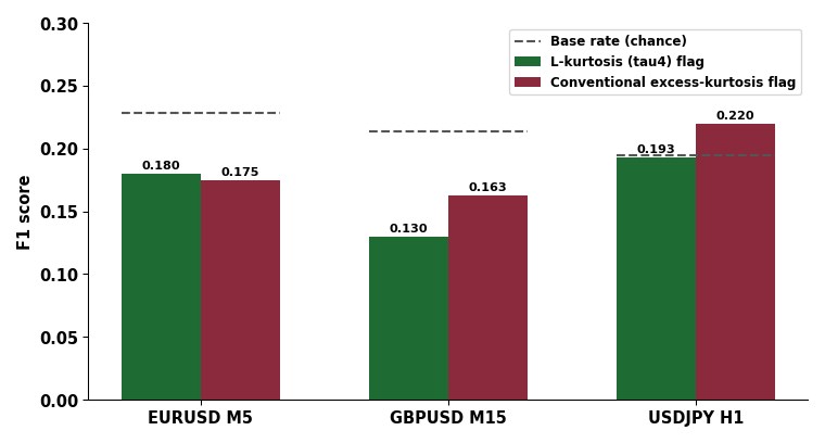
Fig. 2. Real precision/recall/F1 results from the three walk-forward runs, with each pair's base rate marked as a dashed line.
Judged on precision against the base rate – the more relevant comparison for a selective flag – the conventional excess-kurtosis flag is ahead on two of the three pair/timeframe cases, and the tau4 flag is ahead on the third by a narrow margin. This is not the clean sweep a robustness argument alone would predict, and it is reported here exactly as measured rather than reframed around the one pair where the L-moment estimator came out ahead. With only three pairs tested and no formal significance test behind any of these differences (covered further in Limitations), "ahead" here means exactly what the numbers show, nothing stronger.
On GBPUSD M15, tau4's precision (0.170) sits below the base rate (0.214) – on this pair and timeframe, a tau4 spike was, in this specific run, less reliable than simply guessing "yes" every time, while the conventional flag's precision (0.242) sits clearly above it. On USDJPY H1, both flags land above the base rate, with the conventional flag's higher recall (0.208 vs 0.166) catching more of the real large moves at a broadly similar precision. EURUSD M5 is the one pair where tau4 edges out the conventional flag on both precision and F1, though the margin is narrow (F1 0.180 vs 0.175) and well within the kind of gap that three data points and no significance test cannot rule out as noise.
Recall across all three pairs stays low for both flags – no single scalar spike, robust or classical, catches most large moves on its own. That is expected: this validator measures one signal in isolation, with a symmetric two-sided definition of "large move," and was never designed to be a complete entry filter by itself.
The raw counts behind those ratios are worth showing directly, since precision and recall alone can obscure how much data each verdict actually rests on. The script itself reports 4,987 bars walked per pair; of those, 4,928 had a full return window and were logged to CSV, and 4,828 of those also had a fully warmed spike baseline and were the ones actually scored (the remaining 100 are the baseline warm-up period, deliberately excluded from scoring as covered in Limitations). Note too that the forward windows behind these counts overlap by construction, so 4,828 is the number of scored rows, not the number of statistically independent observations behind each ratio – also covered in Limitations:
// EURUSD M5   (1,102 real large moves out of 4,828 scored bars)
tau4:         flagged=631  TP=156  FP=475  TN=3251  FN=946
conventional: flagged=705  TP=158  FP=547  TN=3179  FN=944

// GBPUSD M15  (1,032 real large moves out of 4,828 scored bars)
tau4:         flagged=643  TP=109  FP=534  TN=3262  FN=923
conventional: flagged=524  TP=127  FP=397  TN=3399  FN=905

// USDJPY H1   (942 real large moves out of 4,828 scored bars)
tau4:         flagged=672  TP=156  FP=516  TN=3370  FN=786
conventional: flagged=838  TP=196  FP=642  TN=3244  FN=746
One pattern is consistent across all three cases: the conventional flag fires more often than tau4 on two of three pair/timeframe cases (EURUSD M5, USDJPY H1) and less often on GBPUSD M15, but its true-positive count is higher than tau4's on every single case (158 vs 156, 127 vs 109, 196 vs 156). The conventional estimator is, on this specific task, simply catching more real events in absolute terms across the board – it just does so with a proportionally larger false-positive count on two of the three cases, which is what keeps its precision from separating cleanly from tau4's despite the higher raw hit count.
Limitations and Practical Considerations
The results are highly sensitive to the positive-class base rate and the chosen thresholds. A low event frequency can make precision misleading, while different spike multipliers, window lengths, or forward horizons may change the comparison.
Although L-moments are more resistant to outliers, this does not guarantee better predictive performance.The results cover only three instruments and one parameter configuration (60-bar window, 12-bar horizon, ATR(14), and 1.5-standard-deviation spike threshold).
The validator detects large price movements regardless of direction, without accounting for trading costs. Its adaptive baseline uses non-robust mean and standard deviation estimates. It also requires approximately 160 bars of warm-up and assumes closed-bar evaluation, although CopyRates() includes the current forming bar.
Forward evaluation windows overlap, reducing the effective number of independent observations. Small F1 differences are therefore inconclusive. The study includes neither statistical significance testing nor out-of-sample validation.
Before practical use, the method should be tested across additional instruments, periods, and parameter settings, with robust baselines, directional trading costs, and out-of-sample evaluation.
Conclusion
L-moments compute a genuinely more numerically robust set of shape statistics than the classical Pearson moments – that part of the case holds regardless of any single empirical result, since it follows directly from the PWM formula never raising a deviation to a power. What this article's real walk-forward test adds is a more honest picture of what that numerical robustness does and does not buy: on two of three real pair/timeframe combinations, the classical excess-kurtosis flag was the more precise spike detector, and only on EURUSD M5, by a narrow and statistically untested margin, did tau4 come out ahead. Numerical robustness is not automatically synonymous with better forward signal, and this validator's job is exactly to make that distinction checkable rather than assumed – including checking it against the trivial always-flag baseline, which outscored both estimators on F1 at this precision/recall tradeoff.
The practical takeaway is not "always use tau4 instead of kurtosis" or the reverse – it is that either estimator is only as trustworthy as the threshold defining what counts as the event being predicted, that checking the positive-class base rate before reading any precision number is not optional, and that three overlapping pair/timeframe results are not a basis for a strong general claim either way. The three files in this project give a native, dependency-free way to compute both estimators side by side on the same window and check that for any instrument before relying on either one.
| File | Type | Description |
|---|---|---|
| LMomentsCore.mqh | Include | CLMoments: probability-weighted moments and the PWM-to-L-moment/tau3/tau4 pipeline. |
| ReturnWindowStats.mqh | Include | CReturnWindowStats: rolling circular return window plus the conventional Pearson skew/kurtosis baseline over the same data. |
| LMoment_RegimeValidator.mq5 | Script | CRollingBaseline plus the OnStart walk-forward loop: adaptive spike flags, CSV logging, confusion-matrix scoring, and the plain-language verdict. |
Warning: All rights to these materials are reserved by MetaQuotes Ltd. Copying or reprinting of these materials in whole or in part is prohibited.
This article was written by a user of the site and reflects their personal views. MetaQuotes Ltd is not responsible for the accuracy of the information presented, nor for any consequences resulting from the use of the solutions, strategies or recommendations described.


