Neural Networks in Trading: Recurrent Modeling of Market Micromovements (Encoder)

Introduction

In the world of machine learning, there is a special class of architectural solutions capable not only of analyzing data, but also of sensing its underlying dynamics. Among them, the EV-MGRFlowNet framework holds a special place — the result of meticulous engineering work in which researchers proposed an unconventional method for modeling motion based on event streams. Its introduction marked a significant step forward in the field of computer vision. But the true value of this approach extends beyond that: the principles of working with event data are largely in line with the nature of financial markets, where every trade, price change, or surge in liquidity constitutes its own micro-event.

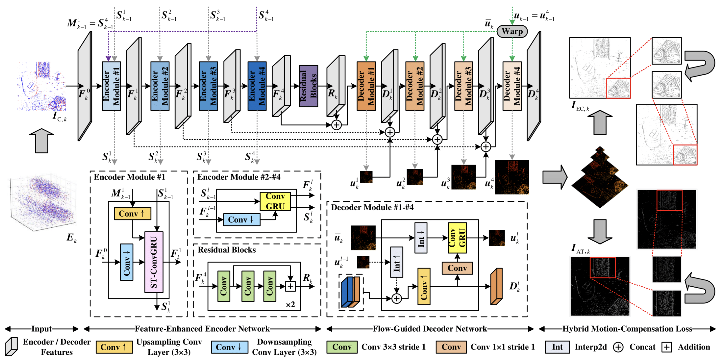
EV-MGRFlowNet is based on a recurrent encoder-decoder architecture built on multi-level refinement of temporal features. The input data — whether it consists of local spikes in the camera's image sensor or market data ticks — passes through a chain of transformations in which the system learns to recognize a coherent pattern of movement. It is in the FERE-Net encoder that the authors implemented one of the key innovations that enables the model to capture subtle temporal dependencies in the data.

The classic ConvGRU updates its memory exclusively along the time axis. Each layer of the model receives its own stream of states and does not interact with other layers along the depth dimension. As a result, low-level representations often lose their connection to the features formed at higher levels. ST-ConvGRU, on the other hand, introduces a mechanism for cross-level coherence. At each time step, a layer's hidden state is updated based not only on its own previous state but also on the signal received from the higher layer. This mechanism significantly deepens the temporal context. The model is able to maintain more complete, consistent representations of motion over time without losing information extracted at other levels of resolution. As a result, FERE-Net generates multilevel temporal maps that preserve both coarse aspects of motion and subtle, barely perceptible details.

The FGD-Net decoder performs the inverse function. It gradually reconstructs the motion map, starting at a coarse level and progressing to increasingly fine detail. This process can be compared to the way an experienced analyst analyzes a market chart. First, it identifies the general direction, then the structure of the impulses and micro-movements that determine the overall behavior of the time series being analyzed. End-to-end consistency between the encoder and decoder allows the framework to generate predictions based on the entire stream.

The HMC-Loss hybrid loss function plays an important role in training the model, as it combines several components related to motion compensation. Each of them is responsible for its own aspect of temporal coherence. One helps align sequential events, another smooths out abrupt transitions, and the third enhances the model's stability. Together, they act as a system of stabilizers that drives the model not merely to minimize error, but also to sense the rhythm of the sequence.

Applying these principles to the financial markets opens up new analytical possibilities. Tick data is essentially the same stream of events, only expressed not in pixels but in changes in price and volume. Tick data is irregular, dynamic, and sensitive to external stimuli. It is precisely this chaotic nature that makes the need for an event-based approach apparent. Where traditional time series obscure information by discretizing the data stream, event-based methods preserve the natural structure of changes. For us, this means that price movements can be viewed as a dynamic chain of events. This chain can be processed within the same paradigm as a data stream from a camera sensor.

Adapting EV-MGRFlowNet to financial data requires an understanding of how its internal components work. Which architectural components are responsible for interpreting events, and which are responsible for motion reconstruction? In this system, the FERE-Net encoder serves as a tool for aggregating micro-events in the market. It converts a sequence of ticks or orders into a multi-layered temporal representation. The FGD-Net decoder, in turn, extracts from this representation the potential direction of movement, the strength of the momentum, or the probability that the trend will continue. Thus, the framework from the field of computer vision flows naturally into the field of market analysis, since in both cases the goal is the same — to observe movement, understand its structure, and predict future developments.

The particular value of this approach lies in its scalability. Since the model is not tied to fixed time intervals, it performs equally well during rapid volatility spikes and periods of calm. This characteristic is particularly important for forecasting, where even the slightest shift in the market phase can be critical. The event-driven model adapts to information density in a natural way, without being artificially forced to fit into interval windows.

Thus, EV-MGRFlowNet is a universal framework for analyzing event streams of any kind. The author's visualization of the framework is shown below.

ST-ConvGRU Module

In the practical section of the previous article, we examined in detail how ST-ConvGRU works and approached its implementation not as a mechanical transcription of equations, but as an engineering problem in which every detail affects the model’s overall ability to recognize motion.

Let me remind you that this module is based on two parallel GRU branches, which function as two interconnected memory channels. The first updates its state based on its own hidden states, while the second incorporates the hidden state of the higher layer, forming a sort of bridge between the layers of the recurrent encoder. This mechanism enhances temporal coherence, allowing the model to retain signals that are inevitably lost between layers in a classical ConvGRU.

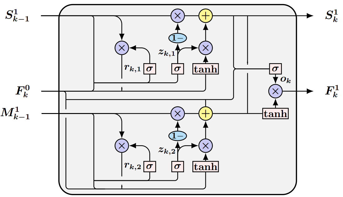
For financial markets, this architecture takes on particular significance. ST-ConvGRU makes it possible to capture patterns that emerge at the level of more complex market contexts: momentum, the inertia of a cluster of large trades, and accumulated shifts in order structure. This model does not just react to yet another price spike — it learns to understand the market conditions that led to that spike.

We also highlighted an important technical aspect. The internal logic of a GRU cell is based on element-wise operations. This paves the way for scaling up computations. If the input data and hidden states are organized properly, any number of GRU cells can be combined into a single unified structure, allowing calculations to be performed in parallel on a GPU. This is critical for us: financial data often arrives at a high frequency, and the model must process long sequences without delay. The transition to OpenCL makes it possible to perform real-time computations without sacrificing either accuracy or the depth of analysis.

In the previous article, we created the necessary OpenCL kernels, thereby laying the foundation for a parallel pipeline. Now comes the key step — setting up the entire system within the main program. Here, we need to integrate the logic of ST-ConvGRU with the temporal memory update mechanism into a single working framework capable of seamlessly processing large arrays of market data. This is the stage where theory is put into practice and the architecture demonstrates its strength under conditions close to real-world trading scenarios.

To implement the ST-ConvGRU functionality, we create a new class, CNeuronSpikeSTConvGRU, which inherits the basic functionality from the CNeuronSpikeActivation object. This object becomes the heart of our system. It does not just process data; it tracks their dynamics over time, accumulating important signals and passing them on to the next layers of the model. The class incorporates a number of support modules that work together as a single mechanism, ensuring a smooth flow of information from input to output.

class CNeuronSpikeSTConvGRU  :  public CNeuronSpikeActivation
  {
protected:
   CNeuronBaseOCL             cConcatenated[2];
   CNeuronMultiWindowsConvOCL cFSM;
   CNeuronBaseOCL             cSM;
   CNeuronConvOCL             cOs;
   CNeuronConvOCL             cOt;
   CNeuronBaseOCL             cFo;
   CNeuronTransposeRCDOCL     cS;
   CNeuronBatchNormOCL        cNorm;
   //---
   virtual bool      GRU(void);
   virtual bool      GRU_grad(void);

   //---
   virtual bool      feedForward(CNeuronBaseOCL *NeuronOCL) override { return false; }
   virtual bool      feedForward(CNeuronBaseOCL *NeuronOCL, CBufferFloat *SecondInput)override;
   virtual bool      updateInputWeights(CNeuronBaseOCL *NeuronOCL) override { return false; }
   virtual bool      updateInputWeights(CNeuronBaseOCL *NeuronOCL, CBufferFloat *second)override;
   virtual bool      calcInputGradients(CNeuronBaseOCL *NeuronOCL) override { return false; }
   virtual bool      calcInputGradients(CNeuronBaseOCL *NeuronOCL, 
                                        CBufferFloat *SecondInput,
                                        CBufferFloat *SecondGradient,
                                        ENUM_ACTIVATION SecondActivation = None) override;

public:
                     CNeuronSpikeSTConvGRU(void) {};
                    ~CNeuronSpikeSTConvGRU(void) {};
   //---
   virtual bool      Init(uint numOutputs, uint myIndex, COpenCLMy *open_cl,
                          uint units, uint &chanels_in[], uint chanels_out,
                          ENUM_OPTIMIZATION optimization_type, uint batch);
   //---
   virtual int       Type(void)   override const   {  return defNeuronSpikeSTConvGRU;   }
   //--- methods for working with files
   virtual bool      Save(int const file_handle) override;
   virtual bool      Load(int const file_handle) override;
   //---
   virtual void      SetOpenCL(COpenCLMy *obj) override;
   virtual bool      Clear(void) override;
   //---
   virtual bool      WeightsUpdate(CNeuronBaseOCL *source, float tau) override;
   //---
   virtual uint      GetChanels(void) const { return cOt.GetFilters(); }
   virtual uint      GetUnits(void) const { return cOt.GetUnits(); }
  };

The Init method is the heart and starting point of the module's operation. It is responsible for building the entire internal structure, allocating channels, and preparing the computational pipeline. Think of it as an engineering blueprint for the model: every part and every block has its own place and function, and only together do they form a well-coordinated machine for processing events.

bool CNeuronSpikeSTConvGRU::Init(uint numOutputs, uint myIndex, COpenCLMy *open_cl,
                                 uint units, uint &chanels_in[], uint chanels_out,
                                 ENUM_OPTIMIZATION optimization_type, uint batch)
  {
   if(chanels_in.Size() != 2)
      return false;

Here, we first check that the parameters received from the user are valid. The input data is expected to arrive in the form of two data streams: the event stream being analyzed and the hidden state of the higher layer. Their dimensions are specified in the chanels_in array. If the size of the array does not match the number of expected data streams, the initialization is aborted.

Control is then passed to the parent class, which handles memory allocation, binding to the OpenCL context, and the basic organization of the neural network. Without this preparation, the module cannot function.

   if(!CNeuronSpikeActivation::Init(numOutputs, myIndex, open_cl, units * chanels_out,
                                    optimization_type, batch))
      return false;

Next, the internal blocks are created. First, we initialize a data concatenation object that combines all the input data into a single feature stream: current events and the hidden states of both this module and the object in the higher layer. At this stage, the data is not yet transformed; it is simply collected for subsequent processing.

//--- Concatenate [2*F0,S0,M0]*Units
   uint index = 0;
   if(!cConcatenated[0].Init(0, index, OpenCL, (2 * chanels_in[0] + chanels_in[1] + chanels_out)*units,
                             optimization, iBatch))
      return false;
   cConcatenated[0].SetActivationFunction(None);

The next block, cFSM, acts as a filter and feature selector, transforming the raw input data and hidden states into a set of components required for the GRU cell to function.

//--- [6*F,3*S,3*M]*Units
   index++;
   uint windows[] = { chanels_in[0], chanels_in[0], chanels_out, chanels_in[1] };
   if(!cFSM.Init(0, index, OpenCL, windows, 3 * chanels_out, units, 1, optimization, iBatch))
      return false;
   cFSM.SetActivationFunction(None);

This is not simply channel concatenation — cFSM is a multi-window convolution object that can simultaneously process multiple information streams and map them to a common dimensionality. Since GRU uses input data and hidden states in three different contexts (updating, state candidates, and forgetting), cFSM immediately creates the necessary number of projections so that each operation can be performed in parallel.

The cSM object receives a concatenated hidden state that combines the contexts of the lower and higher layers.

//--- [S,M]*Units
   index++;
   if(!cSM.Init(0, index, OpenCL, 2 * chanels_out * units, optimization, iBatch))
      return false;
   cSM.SetActivationFunction(None);

Essentially, this is the output of two parallel GRU cells that have already processed the input data and memory signals, forming a consistent representation of the state being analyzed.

Next, we create objects to interpret these results, starting with cConcatenated[1], which combines the hidden states with the input data.

//--- [F,S,M]*Units
   index++;
   if(!cConcatenated[1].Init(0, index, OpenCL, (chanels_in[0] + 2 * chanels_out)*units,
                             optimization, iBatch))
      return false;

This step is necessary to prepare the data for calculating the control signals.

Next comes cOs, the object that generates the output signal oₖ based on the concatenated hidden states and the current input data.

//--- [S]*Units
   index++;
   if(!cOs.Init(0, index, OpenCL, chanels_in[0] + 2 * chanels_out, chanels_in[0] + 2 * chanels_out,
                chanels_out, units, 1, optimization, iBatch))
      return false;
   cOs.SetActivationFunction(SIGMOID);

Here, we use the SIGMOID function to restrict the values to between 0 and 1. This allows each memory unit to decide which portion of the information to retain for the next step and which to filter out. For financial data streams, this resembles a mechanism for selecting which current micro-impulses and higher-layer signals are truly significant for forecasting price movements.

The cOt convolutional layer generates candidates for the new state by producing a prediction based on the updated hidden states.

//--- [S]*Units
   index++;
   if(!cOt.Init(0, index, OpenCL, 2 * chanels_out, 2 * chanels_out, chanels_out, units, 1,
                optimization, iBatch))
      return false;
   cOt.SetActivationFunction(TANH);

We will store the results of element-wise multiplication of the output gates by the corresponding state candidates in the cFo buffer, which holds the output of the ST-ConvGRU module.

//--- [S]*Units
   index++;
   if(!cFo.Init(0, index, OpenCL, chanels_out * units, optimization, iBatch))
      return false;
   cFo.SetActivationFunction(None);

In the context of financial data streams, this is akin to a synthesis of two perspectives: one reflects local changes, while the other reflects the global market context. Concatenation allows the model to simultaneously account for micro-impulses and larger patterns, forming a rich representation of current market dynamics.

The cS object is used to extract the hidden state of the current layer from the concatenated tensor, preparing it for the next time step.

//--- [S]*Units
   index++;
   if(!cS.Init(0, index, OpenCL, units, 2, chanels_out, optimization, iBatch))
      return false;
   cS.SetActivationFunction(None);

Next, we'll deviate slightly from the author's implementation of the module and add spiking activation to the results. Before that, the obtained values pass through the cNorm block, which performs batch normalization. This is critical: normalization stabilizes the signal amplitude, eliminating fluctuations that can occur with long sequences of ticks and large volumes of data.

//--- [S]*Units
   index++;
   if(!cNorm.Init(0, index, OpenCL, Neurons(), iBatch, optimization))
      return false;
   cNorm.SetActivationFunction(None);
//---
   return true;
  }

Only then are the normalized signals fed into the spiking activation layer, where they are converted into events that can be interpreted as discrete pulses in a neural network. In the context of financial data streams, this is similar to identifying key market micro-impulses: each spiking unit signals a significant change in price or volume, allowing the model to focus on the most informative events and effectively accumulate a history of market dynamics for forecasting.

This approach offers a combination of advantages: the accuracy of the authors’ ST-ConvGRU in handling memory and hidden states, as well as spiking selectivity, which helps filter out noise and highlight truly significant events.

When all blocks have been successfully initialized, the method returns true, indicating that the module is ready.

After initializing the object, we move on to the forward pass algorithm, which is implemented in the feedForward method. This method organizes the sequential processing of input data and hidden states, transforming them into the module's updated hidden state and generating a signal for subsequent layers.

bool CNeuronSpikeSTConvGRU::feedForward(CNeuronBaseOCL *NeuronOCL, CBufferFloat *SecondInput)
  {
   if(!NeuronOCL || !SecondInput)
      return false;
//---
   uint Fdimension = cFSM.GetWindow(0);
   uint Sdimension = cS.GetDimension();
   uint Mdimension = cFSM.GetWindow(3);
   uint units = cFSM.GetUnits();

First, the method verifies that the pointers to the source data objects are valid. If even one data stream is missing, the algorithm cannot function, and the process is interrupted.

Next, the dimensions of the key blocks are extracted:

• Fdimension — the dimension of the main data stream window;
• Sdimension — the dimension of the hidden state window of the current layer (S);
• Mdimension — the dimension of the window for the hidden state of the higher layer (M).

These parameters define the framework for the computational process.

Then, sequential data processing begins. First, we extract the hidden state of the current layer obtained during the previous forward pass.

   if(!cS.FeedForward(cSM.AsObject()))
      return false;
   if(!cSM.SwapOutputs())
      return false;

After that, the SwapOutputs method of the cSM object is called to save the hidden states from the previous time step for the backward pass.

The next step is to concatenate the features being analyzed with the hidden states of the current and higher layers. This step generates a single feature tensor that contains all the information needed to process both GRU cells.

   if(!Concat(NeuronOCL.getOutput(), NeuronOCL.getOutput(), cS.getOutput(), SecondInput,
              cConcatenated[0].getOutput(), Fdimension, Fdimension, Sdimension, Mdimension, units))
      return false;

In terms of financial data streams, this is like creating a comprehensive market snapshot at the current tick.

Next, the method of the same name is called on cFSM, performing multi-window convolution and creating projections for the GRU.

   if(!cFSM.FeedForward(cConcatenated[0].AsObject()))
      return false;

Next, the GRU method is called, which updates the hidden states.

   if(!GRU())
      return false;

We concatenate the resulting tensor with the analyzed features of the current state, preparing the data for calculating the output signal and the state candidate.

   if(!Concat(NeuronOCL.getOutput(), cSM.getOutput(), cConcatenated[1].getOutput(),
              Fdimension, 2 * Sdimension, units))
      return false;

Calling the FeedForward method on the cOs and cOt objects generates output gates and candidate outputs for ST-ConvGRU.

   if(!cOs.FeedForward(cConcatenated[1].AsObject()))
      return false;
   if(!cOt.FeedForward(cSM.AsObject()))
      return false;

The ElementMult method then combines them to produce the final result.

   if(!ElementMult(cOs.getOutput(), cOt.getOutput(), cFo.getOutput()))
      return false;

In the final stage, the obtained values are normalized and fed into the spiking activation.

   if(!cNorm.FeedForward(cFo.AsObject()))
      return false;
//---
   return CNeuronSpikeActivation::feedForward(cNorm.AsObject());
  }

In the context of financial data streams, the feedForward method functions as a coordinated analyst. It simultaneously processes current events, takes into account the higher-level context and the history of hidden states, filters out noise, and forms a cumulative view of the market. Each updated hidden state serves as an informative signal for predicting price movements, reflecting both local micropatterns and global trends.

Once we have obtained a forecast using random model parameters, it will, of course, be far from what we want. Therefore, the next step is to organize the training process, which begins by addressing errors. The calcInputGradients method implements error backpropagation through the entire ST-ConvGRU structure.

bool CNeuronSpikeSTConvGRU::calcInputGradients(CNeuronBaseOCL *NeuronOCL,
                                               CBufferFloat *SecondInput,
                                               CBufferFloat *SecondGradient,
                                               ENUM_ACTIVATION SecondActivation = None)
  {
   if(!NeuronOCL || !SecondGradient || !SecondInput)
      return false;
//---
   uint Fdimension = cFSM.GetWindow(0);
   uint Sdimension = cS.GetDimension();
   uint Mdimension = cFSM.GetWindow(3);
   uint units = cFSM.GetUnits();

The algorithm begins by verifying the validity of the pointers to the source data objects. If the main data stream, secondary input, or gradient buffer is missing, the process cannot be executed.

Next, the key parameters are extracted: Fdimension, Sdimension, and Mdimension. This defines the framework of the gradient flow.

Next, the method of the same name in the parent class is called, initiating error propagation from the spiking activation.

   if(!CNeuronSpikeActivation::calcInputGradients(cNorm.AsObject()))
      return false;

The error signal passes through the normalization layer to the ST-ConvGRU output block.

   if(!cFo.CalcHiddenGradients(cNorm.AsObject()))
      return false;

The ElementMultGrad method distributes gradients between the output gates (cOs) and state candidates (cOt), taking their activation functions into account.

   if(!ElementMultGrad(cOs.getOutput(), cOs.getGradient(),
                       cOt.getOutput(), cOt.getGradient(),
                       cFo.getGradient(), cOs.Activation(), cOt.Activation()))
      return false;

This step allows the error to be properly distributed across all memory elements, generating the correct signals for updating the weights.

Next, the gradients pass through cSM, which connects the lower and upper contexts, and through the cConcatenated[1] block, which distributes the errors across the concatenated tensor.

   if(!cSM.CalcHiddenGradients(cOt.AsObject()))
      return false;
   if(!cConcatenated[1].CalcHiddenGradients(cOs.AsObject()))
      return false;
   if(!DeConcat(NeuronOCL.getGradient(), cConcatenated[1].getPrevOutput(),
                cConcatenated[1].getGradient(), Fdimension, 2 * Sdimension, units))
      return false;

DeConcat splits the gradients, returning them to their original blocks, while DeActivation adjusts the values based on the activation functions.

   if(cSM.Activation() != None)
      if(!DeActivation(cSM.getOutput(), cConcatenated[1].getPrevOutput(),
                       cConcatenated[1].getPrevOutput(), cSM.Activation()))
         return false;

The SumAndNormalize method then aggregates gradients from various sources, ensuring stable error propagation through parallel paths.

   if(!SumAndNormilize(cSM.getGradient(), cConcatenated[1].getGradient(), cSM.getGradient(),
                       2 * Sdimension, false, 0, 0, 0, 1))
      return false;

GRU_grad propagates the error within the GRU cells themselves, distributing it between the control signals and the candidate state.

   if(!GRU_grad())
      return false;

After that, the gradients are propagated back to the concatenation tensor cConcatenated[0] via cFSM.

   if(!cConcatenated[0].CalcHiddenGradients(cFSM.AsObject()))
      return false;
   if(!DeConcat(cConcatenated[0].getPrevOutput(), cConcatenated[1].getPrevOutput(),
                cS.getPrevOutput(), SecondGradient, cConcatenated[0].getGradient(),
                Fdimension, Fdimension, Sdimension, Mdimension, units))
      return false;

The DeConcat and DeActivation methods restore the correct signals for the second input and the main NeuronOCL stream.

   if(SecondActivation != None)
      if(!DeActivation(SecondInput, SecondGradient, SecondGradient, SecondActivation))
         return false;

In the final stage, errors at the source data object level are accumulated from various information streams and adjusted using the derivative of the activation function.

   if(!SumAndNormilize(NeuronOCL.getGradient(), cConcatenated[0].getPrevOutput(),
                       NeuronOCL.getGradient(), Fdimension, false, 0, 0, 0, 1) ||
      !SumAndNormilize(NeuronOCL.getGradient(), cConcatenated[1].getPrevOutput(),
                       NeuronOCL.getGradient(), Fdimension, false, 0, 0, 0, 1))
      return false;
   Deactivation(NeuronOCL)
//---
   return true;
  }

In the context of financial data streams, the calcInputGradients method acts as a feedback analyst. It reviews the forecast, compares it with actual market movements, distributes the error across all layers and channels of the module, and adjusts the memory and control signals. Each block of the model receives specific instructions regarding which pieces of information were insufficiently considered or overestimated. This allows us to train the model effectively and improve the accuracy of the predictions.

This mechanism may seem cumbersome, but in multilevel recurrent convolutional architectures, it simply cannot be any other way. Each step affects the next, and even the slightest inaccuracy in gradient distribution instantly leads to a decline in learning performance. The current implementation ensures a strict sequence of calculations and protects the model from such errors, allowing us to move forward with confidence as we fine-tune the parameters.

We will leave the parameter update method updateInputWeights for you to explore on your own. It is intuitive once you understand the structure of the gradient flow. The complete class code, including all helper methods, is provided in the attachment and can serve as a convenient starting point for experimentation and further improvements.

FERE-Net Block

Now that development of the ST-ConvGRU, module is complete, we are approaching a new key milestone: the creation of the encoder, which will serve as the input preprocessing hub for the entire computational chain. Its task is to carefully collect, structure, and transform the data stream so that subsequent layers receive a pre-processed, compact, and informative representation. To do this, we introduce a specialized object: class CNeuronFERENet.

class CNeuronFERENet :  public CNeuronSpikeConvGRU
  {
protected:
   CLayer            cFlow;
   //---
   virtual bool      feedForward(CNeuronBaseOCL *NeuronOCL) override;
   virtual bool      updateInputWeights(CNeuronBaseOCL *NeuronOCL) override;
   virtual bool      calcInputGradients(CNeuronBaseOCL *NeuronOCL) override;

public:
                     CNeuronFERENet(void) {};
                    ~CNeuronFERENet(void) {};
   //---
   virtual bool      Init(uint numOutputs, uint myIndex, COpenCLMy *open_cl,
                          uint units, uint &chanels[],
                          ENUM_OPTIMIZATION optimization_type, uint batch);
   //---
   virtual int       Type(void)   override const   {  return defNeuronFERENet;   }
   //--- methods for working with files
   virtual bool      Save(int const file_handle) override;
   virtual bool      Load(int const file_handle) override;
   //---
   virtual void      SetOpenCL(COpenCLMy *obj) override;
   virtual bool      Clear(void) override;
   //---
   virtual bool      WeightsUpdate(CNeuronBaseOCL *source, float tau) override;
  };

The new class inherits the functional framework of ConvGRU but extends it with its own stream-processing mechanism, implemented using an internal dynamic array called cFlow. It contains the logic that ensures the consistent transformation of the analyzed data during the forward pass, the propagation of gradients during the backward pass, and the updating of parameters.

Initializing the CNeuronFERENet object marks the beginning of a new phase in the construction of our encoder — a phase in which the disparate components begin to come together to form a cohesive computational system.

bool CNeuronFERENet::Init(uint numOutputs, uint myIndex, COpenCLMy *open_cl,
                          uint units, uint &chanels[],
                          ENUM_OPTIMIZATION optimization_type, uint batch)
  {
   uint layers = chanels.Size() - 1;
   if(layers < 2)
      return false;

The process begins with a simple but crucial step. We check the configuration of the supplied array of channel dimensions. This is exactly the kind of situation where classic development principles are like a strict teacher — if the model is not deep enough, there is simply no point in continuing. An encoder must have at least two layers; otherwise, it will not be able to generate complete hidden representations.

After passing the initial check, the object calls the method of the same name in the parent class. This is where the groundwork is laid: buffers are allocated, the OpenCL context is initialized, and optimization parameters are set. You can compare all of this to preparing a workbench before doing delicate manual work — no random tools lying around, everything in its place, and everything strictly tailored to the task at hand.

   if(!CNeuronSpikeConvGRU::Init(numOutputs, myIndex, open_cl, units, chanels[layers - 1],
                                 chanels[layers], optimization_type, batch))
      return false;

Once the basic mechanisms are ready, we begin assembling the encoder's computational pipeline. The cFlow container is cleared and bound to the same OpenCL context.

   cFlow.Clear();
   cFlow.SetOpenCL(OpenCL);

This approach helps avoid unnecessary context switches and achieve high throughput during sequential data processing. Essentially, this creates a path for signals along which all layers of our future encoder will operate.

The first element in this computational pipeline is CNeuronSpikeSTConvGRU. This is not just an input layer — it is a true data filter and organizer that structures the raw data stream into a format suitable for subsequent stages.

   uint index = 0;
   uint windows[] = { chanels[0], chanels[layers] };
   CNeuronSpikeSTConvGRU* st_gru = new CNeuronSpikeSTConvGRU();
   if(!st_gru ||
      !st_gru.Init(0, index, OpenCL, units, windows, chanels[1], optimization, iBatch) ||
      !cFlow.Add(st_gru))
     {
      DeleteObj(st_gru)
      return false;
     }

We provide it with the window sizes, the number of elements, and the dimensionality of the output features. If we picture how the model works, this is the layer that aligns the signal's musical score, turning the raw data stream into fragments neatly arranged as notes in time. After successful initialization, it is added to the computational pipeline. Any failure results in a thorough cleanup of memory — there is no chance of dangling pointers or an undefined state.

Next, the central part of the encoder — the CNeuronSpikeConvGRU chain — begins to take shape. Each layer takes the output of the previous one, progressively condensing the information and deepening its representation. This resembles a sequential process carried out by experts: the first cleans up the signal, the second identifies important structures, and the third forms stable patterns. This cascaded architecture allows the encoder to extract multi-layer hidden dependencies and prepare the data for the final part of the model.

   CNeuronSpikeConvGRU* gru = NULL;
   for(uint i = 1; i < layers - 1; i++)
     {
      CNeuronSpikeConvGRU* gru = new CNeuronSpikeConvGRU();
      if(!gru ||
         !gru.Init(0, index, OpenCL, units, chanels[i], chanels[i + 1], optimization, iBatch) ||
         !cFlow.Add(gru))
        {
         DeleteObj(gru)
         return false;
        }
     }
//---
   return true;
  }

At every step, a new object is created, its initialization is triggered, and if everything goes well, it is woven into the computational pipeline. But as soon as the slightest glitch occurs, we immediately free up resources and halt the process. This strictness is a fundamental characteristic of all stable systems: the computational pipeline must either be fully assembled or not assembled at all.

When the chain is complete and all layers are neatly in place, the method returns a success result. This means that the encoder is ready for operation.

After successful initialization, the model must demonstrate its professional expertise by running through the computational pipeline and forming a stable hidden representation of the data stream being analyzed. That is exactly what the feedForward method does. There is no room for improvisation here. Every step is carefully calibrated, and any deviations immediately halt the process, protecting the model's logic from damage.

bool CNeuronFERENet::feedForward(CNeuronBaseOCL *NeuronOCL)
  {
   CNeuronBaseOCL *prev = NeuronOCL;
   CNeuronBaseOCL *curr = cFlow[0];

At the very beginning, we define two reference variables: prev and curr. The first points to the object whose data will serve as input for the current layer. The second points to the layer to be activated. This pair functions as a transmission mechanism: one element transmits the impulse, while the other receives and converts it.

The first pipeline element, cFlow[0], is retrieved immediately. This is the very same ST-ConvGRU that we set as the input block. It is unusual in that it receives not only the results of the previous layer but also the state of the higher layer as input. This role is fulfilled by the inherited object cH. It serves as a kind of supplementary context that retains a memory of what is happening in the higher layer and allows the layer to handle temporal dependencies more flexibly and with greater foresight.

   if(!curr ||
      !curr.FeedForward(prev, cH.getOutput()))
      return false;
   prev = curr;

This module acts like an experienced analyst who examines data not only in the here and now, but also in light of past trends — and this is particularly valuable when it comes to financial time series.

If something goes wrong, we stop working immediately. But if everything goes well, prev is updated. Now it points to the calculated result, which will be fed to the next layer.

Next, we move on to the central part of the encoder — the ConvGRU cascade stored in cFlow. In the loop from the second layer to the last, each block receives exactly one input — the output of the previous layer, which we carefully pass through the variable prev.

   for(int i = 1; i < cFlow.Total(); i++)
     {
      curr = cFlow[i];
      if(!curr ||
         !curr.FeedForward(prev))
         return false;
      prev = curr;
     }
//---
   return CNeuronSpikeConvGRU::feedForward(prev);
  }

The architecture becomes a well-tuned computational pipeline. The signal passes sequentially through filters that identify local patterns, followed by convolutional-recurrent modules that deepen the model and extract more abstract temporal dependencies.

Each call is a small data-processing operation. Calculating projections, updating hidden states, applying activations, and preparing information for the next layer. Each of these layers is a tool that filters out noise, highlights a trend, or detects a hidden cycle. As a result, the signal emerges from deep within the pipeline in a much more mature and structured form than it was at the input.

Once processing through the entire cFlow pipeline is complete, the last layer in the chain is passed to the method of the same name in the parent class. That is an important detail. Our encoder does not loop back on itself, but instead forwards data to the upper level of the model. This is where the next processing stage begins, which is responsible for integrating the resulting representation into the overall model structure.

Thus, the entire feedForward method acts like a graceful conductor: it takes raw data, passes it through a series of structuring and recurrent transformations, and sends the result to the higher layers, ensuring a clean structure and orderly signals. And all of this is done in a rigorous, coherent manner, without a single unnecessary step — just as a well-designed model intended for the analysis of financial time series should behave.

The encoder's linear structure also works to our advantage in the context of training. Since the forward pass is structured as a strict, sequential chain with no branches, the backward pass follows the same predictable logic. Gradients travel through the same nodes, but in the opposite direction, encountering neither hidden branches nor additional pockets of computation. For a researcher, this convenience is akin to working with classical indicators: if the input signal follows a straight path, the wave propagating back is just as clear and transparent.

We have deliberately avoided overloading this article with details about the backward pass — all the methods strictly follow the familiar pattern and contain no hidden nuances that would require separate, in-depth discussion. Interested readers will easily find the complete class code in the attachment and will be able to study it at their own pace, comparing each operation with the mechanics of a forward pass. This approach allows us to stay focused on the architectural essence of the encoder, without getting sidetracked by repeating already familiar computational patterns.

We have accomplished an impressive amount of work today, and it is time to take a short break. Let's give our thoughts time to settle and our eyes a rest. There is wisdom in a brief pause: a fresh perspective tomorrow will allow us to confidently bring what we have started to its logical conclusion. In the next article, we will continue on this path and carefully complete the implementation of the proposed architecture.

Conclusion

Today's work marked another step toward the practical implementation of the EV-MGRFlowNet architecture using MQL5. We have examined the key elements of ST-ConvGRU, laid the foundation for the encoder, and demonstrated how these mechanisms can be adapted for analyzing market dynamics. As the project progresses, the structure becomes increasingly well-defined, and the model gains the functional depth necessary to handle streaming financial data with confidence. In the next article, we will continue on this path, completing the architecture and moving closer to evaluating the effectiveness of an approach that promises to open up new possibilities for forecasting market movements.

Links

• EV-MGRFlowNet: Motion-Guided Recurrent Network for Unsupervised Event-based Optical Flow with Hybrid Motion-Compensation Loss
• Other articles in this series

Software used in this article

#	Name	Type	Description
1	Study.mq5	Expert Advisor	Expert Advisor for offline model training
2	StudyOnline.mq5	Expert Advisor	Expert Advisor for online model training
3	Test.mq5	Expert Advisor	Expert Advisor for model testing
4	Trajectory.mqh	Class library	Structure describing the system state and model architectures
5	NeuroNet.mqh	Class library	Class library for building a neural network
6	NeuroNet.cl	Library	Code library for an OpenCL program