MetaTrader 5 Machine Learning Blueprint (Part 25): Live Monitoring

Table of Contents

1. Introduction
2. Data, Trades, and Simulation Settings
3. The Sequential-Testing Defect in a Fixed Threshold
4. Wald's SPRT Is Not a Monitor, and a CUSUM Needs a Horizon
5. Choosing the Degraded Win Rate
6. Two Detectors for Two Failure Modes
7. Composing Them: LiveStrategyMonitor
8. Running It on a Real EURUSD Strategy
9. Conclusion
10. Attached Files

Introduction

Beyond its constructors, afml.strategies.learned_strategies.LearnedStrategy exposes generate_signals, get_strategy_name, and get_objective. None of them accepts a trade outcome. Once a strategy is deployed there is no place for a closed trade to go and no object that tracks whether the strategy is still working. The concerns of Part 24 carry over after deployment, where the evidence arrives one trade at a time and the incentive to keep a losing strategy running is strongest.

The obvious fix looks statistical: after every trade, compute the posterior probability that the true win rate has fallen below its historical value, and retire the strategy the first time that probability crosses 95%. The statistic is standard, since a Beta posterior on a Bernoulli win rate is textbook. The procedure built around it is not, and Section 3 measures by how much at this series' own win rate.

This article implements three components in afml.monitoring. First, WinRateSPRT, a sequential probability ratio test with two modes: Wald's terminating test for a one-shot decision on a fixed batch, and Page's reflecting CUSUM for continuous monitoring. Helper functions compute the CUSUM's false-alarm probability over a planned horizon and set its boundary to hold that probability at a chosen level. Second, profit_factor_trend, a resampling trend test on granular profit factor, aimed at a failure mode a win-rate test cannot see. Third, LiveStrategyMonitor, which composes both into the post-deployment interface the pipeline was missing.

The empirical numbers come from two sources: the RSI(14) EURUSD trade list of Part 24, which Section 2 documents in full and the attached script regenerates, and seeded simulations parameterized at that strategy's own win rate. This is the third article in the four-part degradation-avoidance sequence. Part 23 screened the features, Part 24 risk-profiled the backtest, this article watches the strategy after it ships, and Part 26 asks whether the process that produced it would have produced an equally convincing result from noise.

Data, Trades, and Simulation Settings

The trade series

Every real-data result below depends on one trade list. The attachment contains the quote file, the rule that turns it into trades, and the resulting list itself, so a reader can either rerun the rule or start from the trades.

Property	Value
Quote file	EURUSD_H1_time_2018-01-01-2024-12-31.parq (attached; the same file as Part 24), SHA-256 47bebd765c107d4627007ebfcb15ffdb1e3c8be9701ffc2ff46d99560a898fed
Source	EURUSD bid and ask tick history from FundedNext's MetaTrader 5 trade server, aggregated into H1 time bars
Bars	43,103 H1 bars from 2018-01-02 to 2024-12-31, labeled by bar close in broker server time (GMT+2, GMT+3 during daylight saving); bars with no ticks are dropped
Signal	RSI(14) with Wilder smoothing on the mid close; RSI below 30 opens a long, above 70 opens a short
Entry and exit	Entry at the close quote of the bar after the signal bar (ask for a long, bid for a short); exit 20 bars later at the close quote (bid for a long, ask for a short); no new signal until the bar after the exit, so trades never overlap
Sizing	One times notional per trade; the trade return is the P&L as a fraction of notional (pnl_fraction)
Costs	The recorded bid-ask spread only; no commission, swap, or slippage
Execution model	Bar-level Python simulation on H1 close quotes in part25_reproduce.py; the MetaTrader 5 Strategy Tester is not used
Trade list	eurusd_rsi14_trades.csv (attached, and rewritten by the script): 820 trades with entry_time, exit_time, side, and return
Segments	Historical: 466 trades entered in 2018–2021. Live: 354 trades entered in 2022–2024, streamed in order of close time

Two properties of the historical segment matter later. Its win rate is 48.5%, with a 95% interval of 44.0% to 53.0% from 466 trades, so the value the monitor treats as known is itself an estimate. Its average winner is 25.2 basis points of notional and its average loser 25.8, so the break-even win rate is 50.6%, above the realized rate: after the spread, the 2018–2021 segment lost 1.08 basis points per trade on average (profit factor 0.92). The rule was fixed in advance as a test vehicle, and Section 5 returns to what this means for choosing the degraded win rate. Costs move the win and loss counts that the detector sees: a round-turn commission of 0.7 basis points would lower the historical win rate to 47.4% and the live one from 54.5% to 53.4%.

The script writes the trade list, and the remaining code blocks start from it:

import pandas as pd

trades = pd.read_csv("eurusd_rsi14_trades.csv", parse_dates=["entry_time", "exit_time"])
hist = trades[trades["entry_time"] < "2022-01-01"]   # 466 trades, 2018-2021
live = trades[trades["entry_time"] >= "2022-01-01"]  # 354 trades, 2022-2024
historical_win_rate = (hist["return"] > 0).mean()    # 0.485
trade_outcomes = (live["return"] > 0).tolist()       # True for a winning trade
trade_returns = pd.Series(live["return"].to_numpy(),
                          index=pd.DatetimeIndex(live["exit_time"]))

Simulation settings

Every simulation is seeded, and the seeds are fixed in part25_reproduce.py. A run that never crosses a boundary within its horizon is censored: it counts as "not detected" in every rate, and it contributes the horizon to any run-length mean, which then becomes a lower bound. The censored share is reported where it is not zero. Proportions carry 95% Wilson intervals and means carry 95% normal intervals; both describe Monte Carlo error only.

Experiment	Runs	Seed	Trades per run
Posterior threshold on healthy streams (Section 3)	20,000	0	300
CUSUM false alarms and boundary calibration (Section 4)	20,000	2, 1	300
Average run lengths (Section 4)	3,000	0, 3	20,000
Healthy-then-degraded streams (Section 4)	5,000	4	500
Degraded-rate sensitivity (Section 5)	20,000	10–12	3,000
Size of the trend-test nulls (Section 6)	2,000	20	35 periods
Joint behavior of both detectors (Section 7)	2,000	30	354
Profit-factor test after every trade (Section 7)	500	40	354

Two runs of the script on the attached data produce identical output files.

The Sequential-Testing Defect in a Fixed Threshold

The posterior probability that a win rate has degraded below p0, after k wins in n trades under a uniform prior, is the CDF of a Beta(k+1, n−k+1) distribution at p0, the regularized incomplete beta function. deterioration_probability computes exactly this, and it is a sound quantity for a monitoring chart. It is the wrong quantity for a trigger, for a reason that has nothing to do with the statistic itself.

from afml.monitoring import deterioration_probability

posterior = deterioration_probability(k_wins=142, n_trades=300, p0=0.485)
# correct as a number; misleading as a trigger evaluated fresh after every trade

Re-evaluating a fixed threshold on accumulating data turns the procedure into a sequential test. Each additional look is another chance to cross the threshold by chance, even if the true win rate has not changed. The 5% that a 0.95 posterior threshold appears to promise describes a single evaluation, and the procedure that recomputes it after every trade is not a single evaluation.

The simulation uses this series' historical win rate, 48.5%. In 20,000 simulated streams of 300 trades each, with the true win rate fixed at 48.5% throughout, a single look at trade 300 crosses the threshold in 5.2% of streams (95% interval 4.9% to 5.6%). Checking after every trade from the first, the procedure retires the strategy at least once in 33.4% of them (32.8% to 34.1%). The threshold can be repaired: raised to 0.9956, the every-trade procedure fires in 5.2% of a fresh set of healthy streams (4.9% to 5.5%). Section 4 shows what that repair costs in detection, and what a different detector gains at the same false-alarm rate.

False-alarm probability over 300 healthy trades, and detection outcomes around a win-rate break

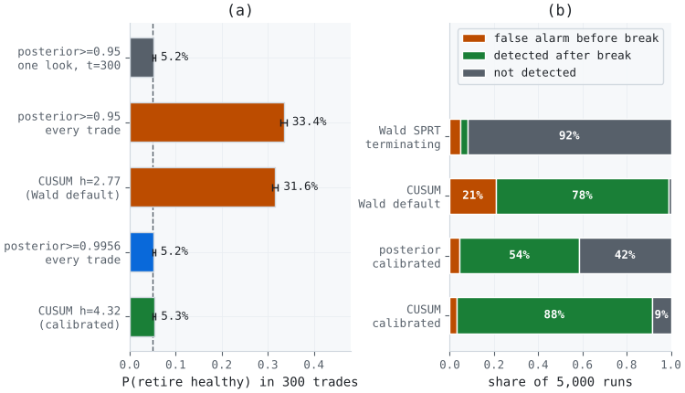
Figure 1. 2-panel illustration of the sequential-testing defect and of detection at a matched false-alarm rate

• Panel (a): the probability of retiring a strategy whose win rate never moves, over 300 trades, for five procedures, with 95% Monte Carlo intervals. Checking the 0.95 posterior after every trade fires in 33.4% of streams, and a CUSUM with the default Wald boundary fires in 31.6%. Raising the posterior threshold to 0.9956, or the CUSUM boundary to 4.32, holds the rate near 5%.
• Panel (b): outcomes across 5,000 simulated runs of 200 healthy trades (48.5%) followed by 300 degraded trades (38.5%), split into false alarms before the break, detections after it, and runs never flagged. Section 4 explains each row.

deterioration_probability remains in the module, with its docstring stating that it is for reporting and for the monitoring chart, not a trigger.

Wald's SPRT Is Not a Monitor, and a CUSUM Needs a Horizon

Wald's sequential probability ratio test addresses the repeated-look problem directly. It tests H0: win rate = p0 against H1: win rate = p1, accumulates a log-likelihood ratio after every trade, and compares it against two boundaries derived from target error rates α and β. Crossing the upper boundary accepts H1 and retires the strategy; crossing the lower boundary accepts H0 and confirms it healthy. Wald's bounds keep the error rates approximately at their targets however often the statistic is inspected.

Applied as a monitor, it fails for a different reason: it is built to reach a decision and then stop. The experiment in Figure 1(b) simulates 200 trades at the healthy win rate (48.5%), then 300 trades at a degraded win rate (38.5%), 5,000 times, and runs each stream through the terminating test.

from afml.monitoring import WinRateSPRT

sprt = WinRateSPRT(p0=0.485, p1=0.385, alpha=0.05, beta=0.20, reflecting=False)
for outcome in trade_outcomes:
    decision = sprt.update(outcome)
    if decision != "continue":
        break  # the decision is final from here on

In 90.9% of the 5,000 runs (90.1% to 91.7%), the terminating test accepts the healthy hypothesis before trade 200, before the break has happened. Having reached a terminal decision, it never revisits it. It detects the later degradation in 3.3% of runs (2.8% to 3.8%). The test is doing what it was built to do; a live monitor needs an answer to a different question.

Page's CUSUM is Wald's SPRT with the lower boundary replaced by a reflecting barrier at zero: WinRateSPRT(…, reflecting=True). Evidence of health drives the statistic toward zero but never past it, so there is no terminal healthy decision and the detector keeps watching. With the default Wald boundary it flags the degradation after the break in 78.3% of the same runs (77.2% to 79.4%). In another 20.7% (19.6% to 21.9%) it fires during the 200 healthy trades, before the break exists.

That false-alarm rate is what the reflecting barrier changes. Over an unbounded horizon a CUSUM fires with probability one, so α is no longer the probability of a false retirement; it is only a boundary parameter. The governing quantities are the average run length to a false alarm, ARL0, the average run length to detection once degraded, ARL1, and, for a deployment of known length, the probability of a false alarm within it.

from afml.monitoring import calibrate_boundary, cusum_run_lengths, false_alarm_probability

rl0 = cusum_run_lengths(0.485, 0.385, true_p=0.485, horizon=20_000, n_sim=3000, seed=0)
rl1 = cusum_run_lengths(0.485, 0.385, true_p=0.385, horizon=20_000, n_sim=3000, seed=0)
fa = false_alarm_probability(0.485, 0.385, horizon=300, seed=2)
h = calibrate_boundary(0.485, 0.385, horizon=300, max_false_alarm=0.05, seed=1)
print(rl0.mean(), rl1.mean(), fa, h)  # 738.1 98.5 0.3156 4.3232

At the default boundary of 2.77, ARL0 is 738 trades (95% interval 713 to 763) and ARL1 is 98.5 (96.2 to 100.8); no run was censored at 20,000 trades. At roughly 120 trades a year, that is one false alarm per six years of healthy trading on average. The average hides the risk over a finite deployment. The run-length distribution is right-skewed (median 510 against the mean of 738), and a healthy strategy is retired within 300 trades with probability 0.32 (95% interval 0.309 to 0.322), and within the 354 trades of Section 8 with probability 0.37. An ARL0 two or three times the planned trade count does not make a false alarm unlikely.

calibrate_boundary searches for the boundary whose false-alarm probability over a planned horizon equals a target. For 300 trades at 5% it returns 4.32, and a simulation with an independent seed gives 5.3% (5.0% to 5.6%). The boundary itself carries Monte Carlo error: the same calibration with seed 10 in Section 5 returns 4.34. The price of calibration is detection speed. ARL1 rises from 99 trades to 173 (169 to 176), which at this strategy's trade rate is about a year and a half of degraded trading before retirement on average.

The comparison that matters is therefore at a matched false-alarm rate, which is what the last two rows of Figure 1(b) show. With both detectors held near 5% over the healthy phase, the repaired posterior threshold detects the break in 53.9% of runs (52.6% to 55.3%) with a median delay of 194 trades. The calibrated CUSUM detects it in 88.4% (87.5% to 89.2%) with a median delay of 119. That gap is the case for the CUSUM in this setting. Error control alone is not, since a posterior threshold can be raised until it has error control too.

A representative run of both detectors, and retirement progress on the real 2022–2024 stream

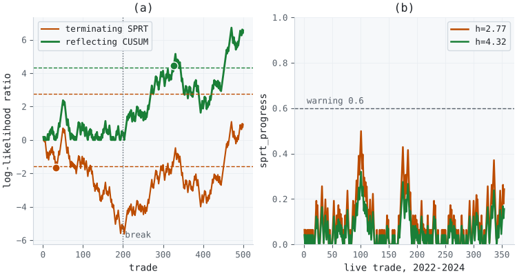
Figure 2. 2-panel illustration of the terminating-versus-reflecting distinction and a real deployment trace

• Panel (a): one simulated run from Figure 1(b), chosen because the calibrated CUSUM's delay is within ten trades of its median. The terminating SPRT (orange) crosses its lower boundary at trade 32 and accepts the healthy hypothesis. The statistic keeps recording afterward, and rises after the break at trade 200, but the decision has latched. The reflecting CUSUM (green) holds near zero through the healthy phase, climbs after the break, and crosses the calibrated boundary of 4.32 at trade 327.
• Panel (b): introduced in Section 8.

The terminating mode is not obsolete. It is appropriate for a one-shot acceptance decision on a fixed batch of trades. The attached regression test asserts that, once decided, the terminating mode holds its verdict through 200 consecutive losses; that behavior is intentional and is not what a live monitor should do.

Choosing the Degraded Win Rate

Every boundary, run length, and delay above is conditional on p1, the degraded win rate the detector is built to find. The SPRT requires it to be stated before deployment; the question is how to choose it. Three inputs bear on the choice: what a given drop costs, how quickly a detector built for it finds it, and how the detector behaves when the true drop differs from the one it was built for.

The economic rule, and why it does not apply here. When the historical win rate is profitable, a natural choice is the break-even win rate, the point below which the strategy loses money on average. With the historical segment's average winner and loser, break-even is 50.6%, above the historical 48.5%. This strategy had no edge after the spread in 2018–2021, so the economic rule says not to deploy it. A monitor cannot repair that; it can only detect a change relative to the behavior it was given. The rest of this section treats the strategy as the test vehicle it is and asks how the choice of p1 plays out.

Cost per point. With winners and losers of the historical sizes, each point of win rate is worth about 0.51 basis points of notional per trade. A ten-point drop therefore costs 5.1 basis points per trade relative to the historical behavior, or about 6.1% of notional per year at 120 trades. The cost of a drop grows linearly with its size, while the number of trades a sequential test needs to detect it grows roughly with the inverse square of its size. That is the trade-off the tables below quantify.

from afml.monitoring import calibrate_boundary, cusum_run_lengths

for p1 in (0.435, 0.385, 0.335):
    h = calibrate_boundary(0.485, p1, horizon=300, max_false_alarm=0.05, seed=10)
    for true_p in (0.435, 0.385, 0.335):
        rl = cusum_run_lengths(0.485, p1, true_p=true_p, horizon=3000, boundary=h, seed=12)
        print(p1, round(h, 2), true_p, (rl <= 300).mean(), rl.mean())

Design drop (p1)	Calibrated boundary	Mean delay at that drop (trades)	Excess loss before detection (% of notional)
5 points (0.435)	2.84	393	10.0
10 points (0.385)	4.34	173	8.8
15 points (0.335)	5.18	96	7.4

Each boundary holds the false-alarm probability near 5% over 300 healthy trades; with the uncalibrated Wald boundary of 2.77, the same three designs would false-alarm in 5.6%, 31.0%, and 56.9% of healthy streams. The excess loss is the per-trade cost of the drop multiplied by the mean delay, uncompounded: a 5-point drop costs half as much per trade as a 10-point drop but takes more than twice as long to find, so it accumulates more loss before detection. The second table crosses each design with each true drop and reports the share of runs detected within 300 degraded trades.

Design drop	True drop 5 points	True drop 10 points	True drop 15 points
5 points	45.4%	93.4%	99.9%
10 points	39.3%	89.9%	99.9%
15 points	33.1%	83.6%	99.5%

The table does not single out ten points. At a matched false-alarm rate, the 5-point design detects a 10-point drop within 300 trades in 93.4% of runs against 89.9% for the 10-point design, and it has the highest chance of catching a 5-point drop (45.4% against 39.3% and 33.1%). It gives up speed against large drops: its median delay on a 15-point drop is 103 trades against 84 for the 15-point design. These figures are for this win rate, a 300-trade calibration horizon, and independent trades.

The rest of the article keeps p1 = 0.385, a 10-point drop, so that Sections 4 and 8 stay comparable. The procedure generalizes: state the per-trade cost of a drop from your own winner and loser sizes, state the false-alarm probability you accept over the horizon you plan to watch, calibrate each candidate p1 to that rate, and choose from the delay and excess-loss columns. A risk limit can be applied to the excess-loss column directly: if a strategy may lose at most a given fraction of notional to an undetected decline, the designs whose expected excess loss exceeds it are ruled out.

Two Detectors for Two Failure Modes

The win-rate detector tracks how often the strategy wins. It fires on a hit-rate collapse. It cannot see a strategy that keeps winning as often as before while its winners get smaller and its losers get bigger, because a test built from win and loss counts carries no information about their size.

profit_factor_trend is aimed at that failure mode. It computes profit factor, gross profit over gross loss, inside non-overlapping calendar periods, then tests whether that granular series is declining. Two choices in the implementation determine its behavior.

Regress the logarithm. A profit factor of 2.0 and one of 0.5 are symmetric departures from break-even: one wins twice what it loses, the other loses twice what it wins. On the raw scale they are not symmetric (1.0 above break-even against 0.5 below), so an untransformed regression gives profitable periods more weight than losing ones. On the log scale they are +0.69 and −0.69.

Choose the null to match the dependence. Profit factor is a ratio of sums, bounded below at zero and right-skewed, so the ordinary least-squares t-distribution for a slope fitted to it is not trustworthy. A resampling null avoids that distributional assumption, but it brings its own. Shuffling the periods gives the exact null distribution of the slope only when the periods are exchangeable under the null, for example independent and identically distributed. Positive serial dependence violates that and makes the shuffled null too narrow. The function therefore offers three nulls: an i.i.d. permutation, a block permutation that shuffles runs of consecutive periods (by default, the cube root of the number of periods, rounded up), and an exhaustive circular shift that keeps the whole dependence structure except at the wrap point. The last two are approximations, and the circular null cannot produce a p-value below 1/n.

from afml.monitoring import granular_profit_factor, profit_factor_trend

pf = granular_profit_factor(trade_returns, freq="ME", min_trades=5)
for null in ("permutation", "block", "circular"):
    trend = profit_factor_trend(pf, n_perm=2000, null=null)
    print(null, trend.slope, trend.p_value, trend.lag1_autocorr)

How much the choice matters depends on the dependence. The table reports how often each null rejects at the 5% level when there is no trend, on 35 periods of log profit factor simulated as an AR(1) process with the dispersion of the real monthly series (standard deviation 0.88), 2,000 series per row.

Lag-one autocorrelation	Permutation	Block (4)	Circular
0.0	5.2%	3.9%	3.2%
0.3	10.5%	4.7%	4.1%
0.6	19.7%	8.8%	5.5%

With independent periods all three hold the 5% level or sit below it; the permutation null is exact there, and the other two are conservative. At an autocorrelation of 0.3 the permutation null rejects about twice as often as it should, and at 0.6 about four times. The block null reduces the excess and the circular null removes most of it in this simulation, at the cost of conservatism when the periods are independent. The intervals on these rates are about ±1 to ±2 percentage points. The practical rule: check the lag-one autocorrelation that TrendResult reports, and when it is materially positive, use the block or circular null, or report all three and act on the most conservative.

The granularity is a real choice, not a default to leave alone. min_trades drops any period with too few trades to produce a stable profit-factor estimate, and a low-frequency strategy can starve a fine granularity of usable periods. Section 8 meets exactly this: weekly periods leave a single usable week, too few to fit any trend, so the switch to monthly periods is forced by the period count rather than chosen from trend results.

Composing Them: LiveStrategyMonitor

LiveStrategyMonitor is the object LearnedStrategy does not have: a place for a closed trade to go, and a running assessment of whether the strategy behind it still works. It runs both detectors, because each is aimed at a failure mode the other cannot see. A win-rate retirement sets the status to "retire". A profit-factor decline sets it to "warning".

from afml.monitoring import LiveStrategyMonitor, calibrate_boundary

# boundary with a 5% false-alarm probability over 300 healthy trades
boundary = calibrate_boundary(0.485, 0.385, horizon=300, seed=1)
monitor = LiveStrategyMonitor(
    historical_win_rate=0.485,
    degraded_win_rate=0.385,    # state it; the default is p0 - 0.10
    retire_boundary=boundary,
    pf_freq="ME",
    pf_alpha=0.005,             # tested once per completed month
    pf_null="permutation",
    strategy_name="eurusd_rsi14_meanrev",
)
for close_time, pnl_fraction in trade_returns.items():
    status = monitor.on_trade_closed(pnl_fraction, close_time)
    if status.status == "retire":
        notify(status.reasons)  # your alerting hook

The profit-factor side has the same repeated-look problem as the posterior threshold. Rerunning the trend test after every closed trade at a level of 0.05 is the natural implementation, and on 500 healthy streams it raised a false warning in 37.8% of them (33.7% to 42.1%). Each stream draws winners and losers from the 2018–2021 trades at the 48.5% win rate and places them on the 2022–2024 close times. The monitor therefore tests only completed periods, so a partial month never enters the regression and the test runs once per month, and its default level is 0.005. With monthly checks over the same three years, the false-warning rate is 25.8% at a level of 0.05 (23.9% to 27.8%) and 5.3% at 0.005 (4.4% to 6.4%). That calibration is specific to this strategy and horizon, and the streams have independent trades, so repeat it for yours.

How the two detectors behave together

The detectors read the same trades, so their outputs are not independent: a run of losses both raises the CUSUM and lowers the profit factor of the month it falls in. They are complementary, in the sense that each is built for a failure the other cannot see. The table measures both properties on 2,000 simulated three-year streams per scenario, using the configuration above and the 354 real close times. In the two degraded scenarios the break occurs at trade 118. The payoff break scales every winner by 0.58, chosen so that it costs the same per trade as the 10-point win-rate drop.

Scenario	Win-rate CUSUM fires	Profit-factor test warns	Both
Healthy throughout	6.0%	5.3%	0.6%
Win rate drops 10 points	83.6%	20.4%	19.0%
Winners shrink, win rate unchanged	6.0%	23.4%	1.9%

Three results follow, each scoped to this configuration and these simulated streams.

• False alarms add up. On healthy streams the monitor raises a retirement or a warning in 10.7% of three-year runs (9.4% to 12.1%), roughly the sum of the two detectors' rates. Both fire together in 0.6% of runs (0.3% to 1.0%), against 0.32% if they were independent. The dependence is positive but small (phi coefficient 0.05).
• The failure modes separate. The win-rate CUSUM detects the win-rate drop in 82.5% of runs after the break, and it fires on the payoff break no more often than its false-alarm rate (6.0%). Only the profit-factor test responds to the payoff break.
• The profit-factor test has low power here. It flags the payoff break in 21.9% of runs (20.2% to 23.8%) within the remaining 236 trades, with a median delay of 114 trades among those it catches. A linear trend fitted to monthly points and tested at a level of 0.005 is a slow instrument for a step change of this size. It is a warning channel for gradual decay, not a substitute for the win-rate test.

The readout an operator watches is sprt_progress: the CUSUM statistic as a fraction of the retirement boundary, bounded in [0, 1] and comparable across strategies with different parameters. monitor.llr_path() plotted against the boundary is the corresponding chart.

Three things are deliberately absent, and the module says so. There is no automatic kill switch: the monitor returns a status and the reasons behind it, and wiring that to order flow is a decision with capital at stake that belongs in the execution layer, where an operator can see it before it fires. There is no un-retirement: the decision latches, and reset() exists for a deliberate refit, never for a bad run. There is no drawdown-based trigger. Part 24 found the 95th-percentile resampled drawdown on this strategy to be 1.49 times the realized one over seven years, so drawdowns from healthy trading vary widely. A drawdown trigger set high enough to spare healthy strategies would react slowly, and one set lower would retire them often. Use Part 24's resampling to set drawdown expectations, and this article's CUSUM to make retirement decisions.

Running It on a Real EURUSD Strategy

The 466 trades entered in 2018–2021 establish historical_win_rate = 0.485. degraded_win_rate is set explicitly to 0.385, ten points lower, with the caveats of Section 5. The remaining 354 trades, entered in 2022–2024, stream through on_trade_closed in order of close time, as though this were a live deployment rather than a second backtest slice.

Figure 2, panel (b), is the resulting sprt_progress trace across all 354 trades, at the default boundary of 2.77 and at the calibrated boundary of 4.32. At the default boundary the trace peaks at 0.50 at trade 101 and ends at 0.24; at the calibrated boundary it peaks at 0.32 and ends at 0.16. Neither reaches the 0.6 warning level. The realized win rate over this stretch is 54.5%, above the historical rate, and the posterior probability that the win rate is below 48.5% ends at 0.012. The monitor reports "no deterioration detected". That means no evidence of a ten-point collapse; it does not establish that the strategy improved, and Section 5 shows that the 10-point design detects a 5-point drop within 300 trades in only 39% of runs.

The profit-factor trend needed one adjustment to run at all. At roughly 120 trades a year, weekly granularity leaves only 1 week in the three-year stream with the five trades granular_profit_factor requires. Monthly granularity yields 35 usable periods. Their lag-one autocorrelation in log profit factor is 0.03, with a standard error of about 0.17 under independence, so the data give no sign of the dependence that would invalidate the permutation null, although 35 points cannot rule out a moderate amount. The three nulls agree. The fitted slope is slightly positive, 0.0176 per month, with p-values of 0.88 (permutation), 0.85 (block), and 0.89 (circular): no evidence of decline. Five permutation seeds move the p-value between 0.87 and 0.89.

The two detectors agree, and the agreement should be read for what it is. Both are computed from the same 354 trades, so they are not independent confirmations, and Section 7 shows their alarms are mildly positively dependent. Each failed to find the failure it is aimed at, a falling hit rate or a shrinking payoff ratio, and Section 7 also shows the profit-factor test would have had a low chance of finding a payoff break of the size considered there.

This is not a claim that the strategy is good. Its 2018–2021 segment lost money after the spread, and Part 24 reported its 2.8% seven-year compounded return and its 14.3% realized drawdown. It is a demonstration of what the monitor is for: distinguishing a strategy that is behaving as it has from one that has stopped working, at a false-alarm rate chosen in advance for the horizon being watched.

Conclusion

Key takeaways, each measured at this strategy's win rate and on the streams described in Section 2:

• Do not use a fixed posterior threshold, recomputed after every trade, as a retirement trigger. On healthy streams it retired the strategy in 33% of 300-trade runs against an apparent 5%. Use the posterior for the chart.
• A terminating SPRT is not a monitor. Applied to a continuous stream it accepted the healthy hypothesis early in 91% of runs and stopped responding to a later break. Use reflecting=True (Page's CUSUM) for anything watched continuously, and reserve the terminating mode for a one-shot decision on a fixed batch.
• A reflecting CUSUM has no false-alarm probability until you name a horizon. With the default Wald boundary it retired a healthy strategy in 32% of 300-trade runs. Compute the false-alarm probability for the planned horizon and set the boundary with calibrate_boundary.
• Compare detectors at a matched false-alarm rate. Near 5% over the healthy phase, the calibrated CUSUM detected a ten-point break in 88% of runs against 54% for a repaired posterior threshold.
• Choose the degraded win rate from cost and delay, not by default. Calibrate each candidate to the same false-alarm rate and compare delay and excess loss; on this strategy a 5-point design detected a 10-point drop as often as the 10-point design and had the highest chance of catching a 5-point drop.
• Match the permutation null to the dependence. The i.i.d. shuffle is exact for exchangeable periods and anti-conservative under positive autocorrelation. Check the lag-one autocorrelation, and use the block or circular null when it is positive.
• Treat the two detectors as complementary, not independent. Their false alarms add up to roughly the sum of the two rates, and their joint firing is mildly positively dependent.
• Every detector checked repeatedly needs the same treatment. The profit-factor test, rerun after every trade, warned falsely on 38% of healthy streams. Test completed periods at a calibrated level.

Part 26 closes the four-part sequence with a question none of the first three tools can answer: whether the search process that produced a strategy's parameters would have produced an equally convincing result from a market with no exploitable structure.

Attached Files

The archive mirrors the terminal's MQL5/Files folder. Extract it into the terminal's data directory and run python part25_reproduce.py EURUSD_H1_time_2018-01-01-2024-12-31.parq --out results from MQL5/Files. It requires Python 3.10 or later with NumPy, pandas, SciPy, and pyarrow; the tests also need pytest, and the figures need matplotlib and Pillow.

	File	Module	Description
1.	deterioration.py	afml.monitoring	deterioration_probability, WinRateSPRT, average_run_length, expected_sample_size, cusum_run_lengths, false_alarm_probability, calibrate_boundary.
2.	profit_factor.py	afml.monitoring	profit_factor, granular_profit_factor, profit_factor_trend with permutation, block, and circular nulls.
3.	monitor.py	afml.monitoring	MonitorStatus, LiveStrategyMonitor.
4.	__init__.py	afml.monitoring	Package exports.
5.	test_monitoring.py, conftest.py	afml.tests	Unit and acceptance tests for the three modules.
6.	part25_reproduce.py	Script	Rebuilds the trade list from the quote file and reproduces every number in this article.
7.	generate_figures.py	Script	Draws Figures 1 and 2 from the script's output.
8.	EURUSD_H1_time_2018-01-01-2024-12-31.parq	Data	EURUSD H1 bid and ask bars, 2018–2024 (Section 2).
9.	eurusd_rsi14_trades.csv	Data	The 820 trades with entry time, exit time, side, and return.

Further Reading

• López de Prado, M. (2018). Advances in Financial Machine Learning. John Wiley & Sons.
• Page, E. S. (1954). Continuous inspection schemes. Biometrika, 41(1/2), 100–115.
• Wald, A. (1945). Sequential tests of statistical hypotheses. The Annals of Mathematical Statistics, 16(2), 117–186.
• Wilson, E. B. (1927). Probable inference, the law of succession, and statistical inference. Journal of the American Statistical Association, 22(158), 209–212.