

Neural Networks in Trading: Iterative Forecast Refinement Models (Conclusion)
 145
 0

Introduction
The market is in no hurry to reveal its intentions. It is constantly in motion — flexible, fluid, and often unpredictable. Every price change is not a random spike, but a reflection of the many interactions that take place between market participants and information streams. And while classical models attempt to capture this moment in a single snapshot, the modern RAFT (Recurrent All-Pairs Field Transforms) approach looks deeper. It doesn't make a prediction just once; instead, it refines it repeatedly, engaging in a dialogue with the data.
This idea seems almost philosophical. We're used to the model producing a result and then stepping aside. RAFT, on the other hand, remains part of the process, much like an experienced analyst who tests his assumptions step by step, comparing each new observation with the overall picture of what is happening. Instead of a straightforward input–output function, a field of interconnections is constructed here, in which each element influences the others. This approach doesn't just improve accuracy — it changes our very understanding of forecasting. The result is not a number, but rather the state of the model — a reflection of its internal alignment with the market.
In the original version, RAFT was used to compute optical flow — an estimate of motion between two image frames. However, if we set aside the technical details, the logic behind the method is surprisingly in line with the objectives of financial analysis. After all, here, too, we have two states — the past and the present. We are trying to figure out where the movement is headed. Quotes take the place of pixels. Price patterns take the place of optical structures. And market snapshots at different points in time take the place of frames. Thus, adapting RAFT to trading tasks is a natural step in the development of ideas for iterative refinement of forecasts.
In our previous articles, we have already laid the groundwork. The first article focused on the concept of multiple iterations and described the framework’s overall architecture. The second analyzed key components, from building the correlation field to the recurrent blocks that control the refinement process. We saw how a model can gradually improve its predictions by returning to the original data and re-testing each hypothesis.
Before moving forward, it is worth taking a moment to reflect on why RAFT, in particular, has been such a significant step forward. Its main strength lies in its ability to model the full field of pairwise interactions. Instead of looking for local correlations, it compares all elements with one another, creating a sort of map of mutual attractions and repulsions. In a financial context, this means that each bar, feature, or indicator is considered not in isolation, but in the context of the entire history and all possible relationships. This gives the forecast stability and the model a capacity for systems thinking.
The next key element is iterative refinement. Unlike single-step neural networks, RAFT repeatedly updates the motion estimate — or, in our case, the prediction. After each iteration, the new information is compared with the overall relationship map, and the model adjusts its direction. This strategy resembles the process of analytical reasoning: first a hypothesis, then testing, refinement, and testing again. As a result, RAFT is able to focus on key patterns without losing context or suffering from overfitting.
The recurrent block plays a special role. Its task is to maintain its internal state — that is, the model's memory — and to control the rate of adaptation. In financial applications, this can be interpreted as an internal confidence management mechanism — that is, the extent to which the model is confident in its current estimate. Should the model revise that estimate, and how should it respond to a change in the market regime? Thus, the recurrent component becomes more than just a technical element. It is a regulator of intuition, maintaining a balance between new data and accumulated experience.
The principle of multiscale processing is no less important. The original RAFT architecture uses pyramid-based compression of feature correlations. At each level, information is aggregated and refined at a different resolution. This principle is particularly relevant to the market. After all, short-term fluctuations and long-term trends exist on different time horizons, but they influence each other. A model capable of accounting for this interaction is closer to reality. It sees both individual movements and the overall rhythm of the market.
Implementing these ideas using MQL5 makes the project particularly valuable. MQL5 provides powerful tools for working with time series and direct access to trading data, while OpenCL opens up possibilities for parallel computing. By combining them, we create a testing ground for evaluating fundamental concepts using real-world data, without losing touch with actual trading practices. Each iteration of the model can be tested in real time.
Another interesting aspect of the RAFT framework is that it is versatile. Its principles — the construction of a field of interactions, iterative refinement, and recurrent memory — are not dependent on any specific field. In trading, these ideas make it possible to build a system that does not just make predictions, but learns to refine them. A system that doesn't rush to a decision but checks its steps. In an era when speed and accuracy determine success in the market, this quality becomes a rare advantage.
An illustration of the RAFT framework, created by the author, is shown below.
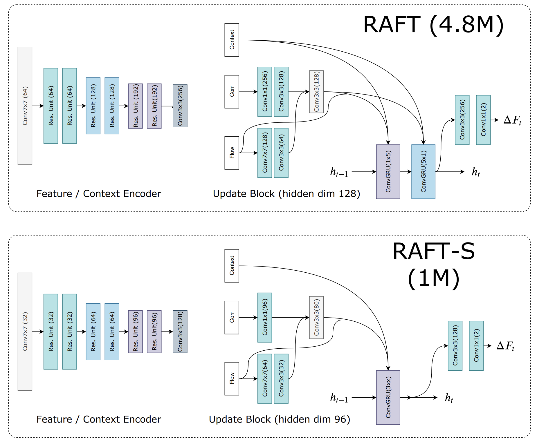
Top-level object
In the previous article, we completed the implementation of the key components of the RAFT framework. Now it is time to move on to the final stage: bringing everything together into a single, cohesive structure, where each component will not only perform its own function but also interact with the others to form a unified mechanism. However, before we get started on this work, it is worth taking a moment to reflect on what exactly we have already accomplished and what questions remain unanswered.
The original RAFT architecture is characterized by elegant symmetry. The same feature encoder architecture is used for two streams: the main stream and the context stream. The main stream encoder analyzes a pair of images, extracting feature maps from them, and then determines the correlations between them. The context encoder works with only one image — the input image — creating a sort of foundation from which the prediction begins. It is this fundamental division of roles that makes the RAFT architecture so robust: one stream is responsible for monitoring changes, while the other is responsible for maintaining the anchor point.
But in the world of finance, things are much more fluid. While frames in computer vision capture a sequence of events with clear boundaries, the market knows no pauses. It does not wait for the model to take a snapshot; it flows continuously. It flows from one state to another, like a river after rain, changing course as it is influenced by new streams of information. And this is where the idea of a fixed context starts to falter. It is impossible to freeze the state of the market in order to base a forecast on it. Something that was relevant just a minute ago may lose its meaning an hour from now.
We have already encountered a similar problem when discussing the use of a fixed initial state in time series forecasting problems. The solution then emerged naturally — we introduced a stack of historical states, which allowed the model to rely not on a single point in time but on an entire sequence, thereby creating a dynamic correlation matrix. This approach made it possible to see the market not as a static snapshot, but in motion, observing how the past interacts with the present.
However, when working with the context stream, things get even more interesting. Context is not just supplementary information. It is an understanding of the current market regime itself. And regimes, as we know, are fickle. Volatility rises, liquidity shifts, and correlations between assets strengthen and then disappear. To freeze the context under such conditions is to condemn the model to blindness. On the other hand, attempting to track context using a history stack leads to excessive complexity and reduced performance. We would end up with a cumbersome structure that loses the main advantage of RAFT — the speed and efficiency of its iterations.
So we need to look for another way — one that is more natural and more flexible. An approach in which the model itself is capable of understanding how the context changes and updating it without external intervention. The idea is simple yet profound: to supplement the contextual encoder with a recurrent block that will track the state of the market in real time. Such a block will be able to remember recent changes, identify recurring patterns, and adjust the context as new data becomes available.
This solution essentially makes the model self-tuning. Context ceases to be an external parameter — it becomes an internal state of the system, living and breathing alongside the market. The model gains the ability not merely to react to input data, but to adapt — that is, to meaningfully adjust its perception of what is happening.
If you will, a recurrent block acts like an analyst's short-term memory: it remembers what happened recently, but is not burdened by the entire history. It stays focused on what is currently relevant, allowing the forecast to remain accurate even amid rapidly changing market dynamics.
This is an important step forward. We are moving from mechanically constructing an architecture to purposefully modeling adaptive behavior. After all, in trading, it is not just about predicting price movements — it is about understanding why they change and being able to adapt to the new market regime. A recurrent contextual encoder will enable the RAFT framework to move closer to this goal.
We implement the proposed ideas in the CNeuronRAFT object, which serves as the central component of our implementation. It is here that all the key components of the framework — the encoders, correlation block, recurrent mechanism, and residual connections — converge into a single structure, forming the dynamic core of the model.
class CNeuronRAFT :  public CNeuronSpikeActivation
  {
protected:
   CLayer                              cEncoder;
   CLayer                              cContext;
   CLayer                              cCorrelation;
   CNeuronBaseOCL                      cConcatenated;
   CNeuronSpikeConvGRU2D               cGRU;
   CNeuronSpikeResNeXtResidual         cResidual;
   CLayer                              cG;
   //---
   virtual bool      feedForward(CNeuronBaseOCL *NeuronOCL) override;
   virtual bool      updateInputWeights(CNeuronBaseOCL *NeuronOCL) override;
   virtual bool      calcInputGradients(CNeuronBaseOCL *NeuronOCL) override;

public:
                     CNeuronRAFT(void) {};
                    ~CNeuronRAFT(void) {};
   //---
   virtual bool      Init(uint numOutputs, uint myIndex, COpenCLMy *open_cl,
                          uint &units[], uint &chanels[], uint group_size,
                          uint groups, uint stack_size, uint levels,
                          ENUM_OPTIMIZATION optimization_type, uint batch);
   //---
   virtual int       Type(void)   override const   {  return defNeuronRAFT;   }
   //--- methods for working with files
   virtual bool      Save(int const file_handle) override;
   virtual bool      Load(int const file_handle) override;
   //---
   virtual bool      WeightsUpdate(CNeuronBaseOCL *source, float tau) override;
   //---
   virtual void      SetOpenCL(COpenCLMy *obj) override;
   virtual void      TrainMode(bool flag) override;
   virtual bool      Clear(void) override;
  };
The structure shown here is not just a collection of objects. It is an architectural ecosystem in which each component plays a role in the overall dynamics.
cEncoder is responsible for the initial extraction of features from the source data. This is a counterpart of the visual encoder in the original RAFT, adapted for financial time series. It transforms a stream of prices and indicator readings into a compact, multidimensional representation, where each coordinate is not a number but a meaningful component of market movement.
cContext creates a context stream. Its architecture is complemented by a recurrent module designed to track the evolution of the market state over time. Thanks to this module, the context is no longer static; it “breathes,” responding to new events and smoothly adapting along with the market, enabling the model to retain a short-term memory of market dynamics.
Next comes cCorrelation, which constructs a matrix of interrelationships between features. That very field of interactions on which the entire RAFT philosophy is based. Here, the features of the current state are compared with a historical data stack accumulated over previous periods. A correlation field is constructed — the very foundation that allows RAFT to capture local shifts and the overall dynamics of processes.
The cConcatenated component combines the outputs of the encoder and the correlation module with the updated context, preparing them for input to the cGRU recurrent block. This module is responsible for iteratively refining the forecast. It evaluates the difference between the previous and current states, makes adjustments, and thereby brings the model closer to a more accurate solution.
The cResidual module acts as a stabilizing element. Rather than propagating gradients as classical residual networks do, it ensures consistency across iterations and prevents feature drift during repeated updates. It is important to understand the fundamental difference between RAFT and traditional forecasting models. The algorithm does not predict the new state directly, but rather generates a feature delta — a refinement that describes the change in the current state. Adding this predicted delta to the original data gives us the desired result.
The authors of the RAFT framework deliberately do not propagate the error gradient along the stream of residual connections. The initial state is considered a fait accompli and cannot be adjusted. Optimization propagates only through the streams being updated — via the correlation and recurrent blocks. This approach makes training stable, prevents backward distortion of the input data, and allows the model to focus on the dynamics of change.
The cG component is the final data processing block, which generates the final map of forecast values. This is where all the model paths converge, and the result of each iteration becomes the input for the next refinement step.
All internal components of a new object are initialized in the Init method. This stage can be compared to the moment when an orchestra gathers before a performance — every instrument must be tuned, and the conductor must be ready to set the tempo. It is here that the entire ensemble of neural blocks is created and coordinated, laying the foundation for the model's coherent dynamics.
bool CNeuronRAFT::Init(uint numOutputs, uint myIndex, COpenCLMy *open_cl,
                       uint &units[], uint &chanels[], uint group_size,
                       uint groups, uint stack_size, uint levels,
                       ENUM_OPTIMIZATION optimization_type, uint batch)
  {
   if(units.Size() != chanels.Size())
      return false;
   uint layers = units.Size() - 1;
   if(!CNeuronSpikeActivation::Init(numOutputs, myIndex, open_cl,
                units[layers]*chanels[layers], optimization_type, batch))
      return false;
The procedure begins by validating the supplied parameters and calling the parent class's initialization method. Next, all the main building blocks of the framework are created: the encoders, the correlation module, the recurrent unit, and the stabilizing residual connection block.
The two-stream structure — cEncoder and cContext — is created first. The CNeuronSpikeResNeXtBlock layers responsible for sequential feature extraction are created in a loop.
   int index = 0;
   CNeuronSpikeResNeXtBlock*           resblock = NULL;
   CNeuronSpikeConvGRU2D*              gru = NULL;
   CNeuronMultiScaleStackCorrelation*  correlation = NULL;
   CNeuronBaseOCL*                     neuron = NULL;
   CNeuronBatchNormOCL*                norm = NULL;
//---
   cEncoder.Clear();
   cContext.Clear();
   cCorrelation.Clear();
   cG.Clear();
   cEncoder.SetOpenCL(OpenCL);
   cContext.SetOpenCL(OpenCL);
   cCorrelation.SetOpenCL(OpenCL);
   cG.SetOpenCL(OpenCL);
//---
   for(uint i = 0; i < layers; i++)
     {
      resblock = new CNeuronSpikeResNeXtBlock();
      if(!resblock ||
         !resblock.Init(0, index, OpenCL, chanels[i], chanels[i + 1], units[i], units[i + 1],
                                                 group_size, groups, optimization, iBatch) ||
         !cEncoder.Add(resblock))
        {
         DeleteObj(resblock)
         return false;
        }
      index++;
      resblock = new CNeuronSpikeResNeXtBlock();
      if(!resblock ||
         !resblock.Init(0, index, OpenCL, chanels[i], chanels[i + 1], units[i], units[i + 1],
                                                 group_size, groups, optimization, iBatch) ||
         !cContext.Add(resblock))
        {
         DeleteObj(resblock)
         return false;
        }
      index++;
     }
The cEncoder stream analyzes features of the current state, while cContext constructs an adaptive context space, supplemented by the CNeuronSpikeConvGRU2D recurrent block. This GRU module enables the framework to track temporal dynamics and adjust the context without a fixed state — a crucial feature when working with continuous market data.
   gru = new CNeuronSpikeConvGRU2D();
   if(!gru ||
      !gru.Init(0, index, OpenCL, units[layers], chanels[layers], chanels[layers], optimization, iBatch) ||
      !cContext.Add(gru))
     {
      DeleteObj(gru)
      return false;
     }
   index++;
Next, the CNeuronMultiScaleStackCorrelation module is created, which generates a correlation matrix between the features of the current state and the historical data stack. This is the central element of the architecture — an analogue of a computational force field in which the relationship between past and present emerges.
   correlation = new CNeuronMultiScaleStackCorrelation();
   if(!correlation ||
      !correlation.Init(0, index, OpenCL, stack_size, chanels[layers], units[layers], levels,
                                                                     optimization, iBatch) ||
      !cCorrelation.Add(correlation))
     {
      DeleteObj(correlation)
      return false;
     }
   index++;
   resblock = new CNeuronSpikeResNeXtBlock();
   if(!resblock ||
      !resblock.Init(0, index, OpenCL, correlation.Neurons() / units[layers], chanels[layers],
                    units[layers], units[layers], group_size, groups, optimization, iBatch) ||
      !cCorrelation.Add(resblock))
     {
      DeleteObj(resblock)
      return false;
     }
   index++;
A CNeuronSpikeResNeXtBlock layer is added to the block's output to enhance the model's selectivity toward the most significant features.
After the correlation field generation block, a concatenation node, cConcatenated, is created to combine the outputs of the three streams — features, context, and correlations — into a single tensor.
   if(!cConcatenated.Init(0, index, OpenCL, 3 * chanels[layers]*units[layers], optimization, iBatch))
      return false;
   index++;
The data is then passed to cGRU, where the forecast delta is refined iteratively.
   if(!cGRU.Init(0, index, OpenCL, units[layers], 3 * chanels[layers], chanels[layers], optimization, iBatch))
      return false;
   index++;
Next, the cResidual stabilization module is initialized. Its purpose is to maintain the structure of the feature space in a stable state over multiple iterations. Unlike in classical residual connections, there is no backpropagation of the gradient here — the baseline state is not adjusted but is used as a reference point to which the feature delta computed by the model is added.
   if(!cResidual.Init(0, index, OpenCL, chanels[0], chanels[layers], units[0], units[layers], optimization, iBatch))
      return false;
   index++;
The final cG block integrates everything into a cohesive system, normalizing the output stream and preparing it for transmission to the next level. This is also where auxiliary objects are created — the base neuron and the CNeuronBatchNormOCL normalization layer, which is responsible for stabilizing the output distribution.
   neuron = new CNeuronBaseOCL();
   if(!neuron ||
      !neuron.Init(0, index, OpenCL, Neurons(), optimization, iBatch) ||
      !cG.Add(neuron))
     {
      DeleteObj(neuron)
      return false;
     }
   neuron.SetActivationFunction(None);
   if(!neuron.SetGradient(cGRU.getGradient(), true) ||
      !cResidual.SetGradient(cGRU.getGradient(), true))
      return false;
//---
   index++;
   norm = new CNeuronBatchNormOCL();
   if(!norm ||
      !norm.Init(0, index, OpenCL, Neurons(), iBatch, optimization) ||
      !cG.Add(norm))
     {
      DeleteObj(norm)
      return false;
     }
//---
   return true;
  }
Thus, the initialization method establishes a logical sequence of computational steps. Each module has a specific purpose: feature extraction, correlation construction, recurrent context refinement, and predictive delta generation. All of these elements come together to form a unified framework, ready for training in real-world market conditions.
The forward pass algorithm is implemented in the feedForward method. This is not just a computational cycle — it is a living process. This is where the model comes to life and begins to get a feel for the market. Each block plays its own role, and together they paint a dynamic picture of future changes.
bool CNeuronRAFT::feedForward(CNeuronBaseOCL *NeuronOCL)
  {
   if(!cResidual.FeedForward(NeuronOCL))
      return false;
The process begins with the cResidual block. You can think of it as a solid foundation or an anchor. It records the current state of the features, establishing a baseline for all subsequent changes.
The next step is the main feature stream, cEncoder. Each ResNeXt block here is like a meticulous researcher who scans the market layer by layer, identifying important patterns and relationships. The output provides a snapshot of the current state — complete and detailed, like a panoramic map of the market at this very moment.
   CNeuronBaseOCL* current = NULL;
   CNeuronBaseOCL* prev = NeuronOCL;
   for(int i = 0; i < cEncoder.Total(); i++)
     {
      current = cEncoder[i];
      if(!current ||
         !current. Feedforward(prev))
         return false;
      prev = current;
     }
The context stream cContext runs in parallel. While the encoder captures a moment, the context stream acts as an observer that remembers the past and recognizes trends. Its recurrent GRU block tracks how the market has changed over the most recent steps and adjusts the forecast accordingly. Context lives and breathes alongside the market, ensuring that the model continuously adapts.
   prev = NeuronOCL;
   for(int i = 0; i < cContext.Total(); i++)
     {
      current = cContext[i];
      if(!current ||
         !current. Feedforward(prev))
         return false;
      prev = current;
     }
Next, the encoder's output is passed to the cCorrelation block. Here, they are added to the history stack of market states, and a multiscale correlation matrix between features is generated. You can think of it as a strategic map, where each point shows how yesterday's events influence today's. It is here that the model uncovers hidden patterns and identifies the strength and direction of market movement.
   prev = cEncoder[-1];
   for(int i = 0; i < cCorrelation.Total(); i++)
     {
      current = cCorrelation[i];
      if(!current ||
         !current. Feedforward(prev))
         return false;
      prev = current;
     }
All three streams — encoder, context, and correlations — are combined in the cConcatenated node. It is like a command center where all the intelligence is gathered. Here, the signal is consolidated before being sent for refinement.
   uint units = cGRU.GetUnits();
   if(!Concat(cEncoder[-1].getOutput(), cContext[-1].getOutput(), cCorrelation[-1].getOutput(),
              cConcatenated.getOutput(), cEncoder[-1].Neurons() / units, cContext[-1].Neurons() / units,
              cCorrelation[-1].Neurons() / units, units))
      return false;
The cGRU recurrent block acts as the commander at this stage. It analyzes the aggregate signal and calculates the feature delta — the predicted change that is added to the initial state to form the final forecast.
   if(!cGRU.FeedForward(cConcatenated.AsObject()))
      return false;
//---
   current = cG[0];
   if(!current ||
      !SumAndNormilize(cGRU.getOutput(), cResidual.getOutput(), current.getOutput(),
                       cGRU.GetChanels(), false, 0, 0, 0, 1))
      return false;
The signal is then sent to the cG block, where it is summed with the residual connection output and normalized. You can think of it as carefully balancing a set of scales — all streams are synchronized, and offsets and noise are eliminated, ensuring the stability of the forecast. Passing sequentially through all layers of cG completes the process of generating results, which now reflect not a static state but a dynamically refined picture of the market.
   prev = current;
   for(int i = 1; i < cG.Total(); i++)
     {
      current = cG[i];
      if(!current ||
         !current. Feedforward(prev))
         return false;
      prev = current;
     }
//---
   return CNeuronSpikeActivation::feedforward(prev);
  }
As a result, feedForward transforms the analyzed data into a living projection of changes, where each block functions as a separate analyst. But together, they form a team capable of identifying trends, anticipating market movements, and adapting to a changing market environment. The model does not attempt to predict the future directly — it calculates the delta and refines the picture step by step, allowing the forecast to be realistic and robust.
Once the forecast has been generated, the next key step is to distribute the error gradient. We implemented it in the calcInputGradients method. If a forward pass can be likened to an orchestra performing a piece, then backpropagation is like a conductor who evaluates each instrument and adjusts its sound so that the entire ensemble performs accurately.
bool CNeuronRAFT::calcInputGradients(CNeuronBaseOCL *NeuronOCL)
  {
   if(!NeuronOCL)
      return false;
//---
   if(!CNeuronSpikeActivation::calcInputGradients(cG[-1]))
      return false;
The method begins by verifying that the pointer to the NeuronOCL source data object is valid. Without it, the model will not be able to distribute the gradients correctly, and the entire process will come to a halt — just as if an orchestra were left without a score.
Next, the parent class method of the same name is called to establish the starting point for backpropagation. You could say this is the metronome's first beat: the gradients begin to flow through the chain of cG components, from the last one to the first.
   CNeuronBaseOCL* current = NULL;
   CNeuronBaseOCL* next = cG[-1];
   for(int i = cG.Total() - 2; i >= 0; i--)
     {
      current = cG[i];
      if(!current ||
         !current.CalcHiddenGradients(next))
         return false;
      next = current;
     }
The loop iterates over the elements of the cG module in reverse order. Each layer receives a signal from the next one, carefully propagating the error. This process resembles the steps taken by an experienced analyst who evaluates each level of the model by comparing the forecast with actual results.
After the cG layers, the gradient is passed to the cResidual block. Here, the error is distributed relative to the initial state, treating it as an unchanging fact. This is the key point: the base features are not modified, but rather serve as the basis for calculating adjustments.
   if(!NeuronOCL.CalcHiddenGradients(cResidual.AsObject()))
      return false;
The gradients are then fed into the cConcatenated concatenation node. From there, they split into three streams: cEncoder, cContext, and cCorrelation. This step can be thought of as an instruction that assigns tasks to three analysts: each is given their own portion of data to process.
   if(!cConcatenated.CalcHiddenGradients(cGRU.AsObject()))
      return false;
   uint units = cGRU.GetChanels();
   if(!DeConcat(cEncoder[-1].getGradient(), cContext[-1].getGradient(), cCorrelation[-1].getGradient(),
                cConcatenated.getGradient(), cEncoder[-1].Neurons() / units, cContext[-1].Neurons() / units,
                cCorrelation[-1].Neurons() / units, units))
      return false;
The next block is cCorrelation. The loop iterates over the layers in reverse order, with each layer adjusting its gradient based on the signal from the next layer. In this section, the model examines how the interaction between current and historical features influenced the final forecast.
   next = cCorrelation[-1];
   for(int i = cCorrelation.Total() - 2; i >= 0; i--)
     {
      current = cCorrelation[i];
      if(!current ||
         !current.CalcHiddenGradients(next))
         return false;
      next = current;
     }
The gradient is then sent to the cEncoder encoder. There is an interesting feature here. The encoder receives error gradients via two data streams. It has already received some information during the deconcatenation of the recurrent block's error gradients. To avoid losing the stored values, the encoder's final layer temporarily saves a pointer to the gradient buffer in a local variable (temp) and uses a free buffer in its place. Next, we compute the gradients along the correlation module path and add them to the stored values.
   current = cEncoder[-1];
   if(!current)
      return false;
   CBufferFloat* temp = current.getGradient();
   if(!current.SetGradient(current.getPrevOutput(), false) ||
      !current.CalcHiddenGradients(next) ||
      !SumAndNormilize(temp, current.getGradient(), temp, temp.Total() / units, false, 0, 0, 0, 1) ||
      !current.SetGradient(temp, false))
      return false;
Next, we reset the buffer pointers to their original state, and the gradients propagate through all the remaining encoder layers.
   next = current;
   for(int i = cEncoder.Total() - 2; i >= 0; i--)
     {
      current = cEncoder[i];
      if(!current ||
         !current.CalcHiddenGradients(next))
         return false;
      next = current;
     }
   if(!NeuronOCL.CalcHiddenGradients(next))
      return false;
After processing the encoder, we move on to the context stream cContext. The loop iterates over the components in reverse order.
   next = cContext[-1];
   for(int i = cContext.Total() - 2; i >= 0; i--)
     {
      current = cContext[i];
      if(!current ||
         !current.CalcHiddenGradients(next))
         return false;
      next = current;
     }
The final operation is to pass the gradients to the source data object NeuronOCL, where the gradients from the two data streams are also carefully summed.
   temp = NeuronOCL.getGradient();
   if(!NeuronOCL.SetGradient(NeuronOCL.getPrevOutput(), false) ||
      !NeuronOCL.CalcHiddenGradients(next) ||
      !SumAndNormilize(temp, NeuronOCL.getGradient(), temp, 1, false, 0, 0, 0, 1) ||
      !NeuronOCL.SetGradient(temp, false))
      return false;
//---
   return true;
  }
As a result, the calcInputGradients method carefully distributes the error throughout the object's architecture — from the output level to the encoder, context, and correlations — adjusting only those parts that are trainable. Each block plays its own role: encoders analyze local features, context takes history into account, correlations capture relationships between elements, and residual blocks ensure the stability of the entire structure. This approach ensures that training proceeds effectively and without distorting the initial states, while preserving the model's dynamic behavior that we observed during the forward pass.
The final stage is parameter optimization — this is where the model adjusts its internal weights to make predictions more accurate. The algorithm is implemented in the updateInputWeights method, which can be compared to tuning all the instruments after a rehearsal.
bool CNeuronRAFT::updateInputWeights(CNeuronBaseOCL *NeuronOCL)
  {
   if(!cResidual.UpdateInputWeights(NeuronOCL))
      return false;
The process begins with the optimization of the residual block, cResidual. It adjusts its parameters while maintaining a stable anchor point for the entire architecture.
Next, the weights are adjusted in the main encoder stream cEncoder. Each layer sequentially receives a signal from the previous block and updates its parameters. You can think of it as a team of researchers who, after receiving feedback, refine their tools to improve the quality of feature extraction on the next pass.
   CNeuronBaseOCL* current = NULL;
   CNeuronBaseOCL* prev = NeuronOCL;
   for(int i = 0; i < cEncoder.Total(); i++)
     {
      current = cEncoder[i];
      if(!current ||
         !current.UpdateInputWeights(prev))
         return false;
      prev = current;
     }
The context stream cContext is updated in the same way. Here, the recurrent GRU uses accumulated gradients to adjust the weights, taking into account temporal dynamics. Each context layer adjusts the influence of past states on current forecasts, allowing the model to respond more flexibly to market variability.
   prev = NeuronOCL;
   for(int i = 0; i < cContext.Total(); i++)
     {
      current = cContext[i];
      if(!current ||
         !current.UpdateInputWeights(prev))
         return false;
      prev = current;
     }
Next, optimization proceeds through the correlation block cCorrelation. Each layer adjusts its parameters based on the signals, improving the accuracy of the interaction matrix between current and historical features. In this way, the model learns to identify the most significant relationships and take past trends into account more accurately.
   prev = cEncoder[-1];
   for(int i = 0; i < cCorrelation.Total(); i++)
     {
      current = cCorrelation[i];
      if(!current ||
         !current.UpdateInputWeights(prev))
         return false;
      prev = current;
     }
The cGRU recurrent node also updates its weights based on the concatenated tensor cConcatenated. A key refinement takes place here: the GRU parameters are adjusted so that the computed feature delta reflects changes in the current state as accurately as possible.
   if(!cGRU.UpdateInputWeights(cConcatenated.AsObject()))
      return false;
Finally, the cG block updates all its layers sequentially, combining the effects of correlations, context, and the direct feature stream, and normalizes the output signal. This final step ensures that every component of the model is synchronized and ready for the next forward pass.
   prev = cG[0];
   for(int i = 1; i < cG.Total(); i++)
     {
      current = cG[i];
      if(!current ||
         !current.UpdateInputWeights(prev))
         return false;
      prev = current;
     }
//---
   return CNeuronSpikeActivation::updateInputWeights(prev);
  }
Finally, the parent class method of the same name is called to complete the optimization cycle. As a result, the weights of all components have been updated, and the model is ready for the next training step or for making predictions on new data.
The attachment contains the complete source code for the object, including detailed implementations of all its methods, showing the inner workings of RAFT.
Model Architecture
We have completed work on building the key components of the RAFT framework and are now moving on to designing the architecture of the trainable models. As before, our goal is to create a trading system capable of independently developing a strategy and executing trades in the market.
To train the models, we use the Actor-Critic approach, integrating the capabilities of RAFT directly into the environment state encoder. This approach allows the model not only to respond to current features, but also to take into account their dynamics and interrelationships, as identified by the framework. At the same time, we use the STFS module to select the most significant features, which allows the model to focus on those aspects that actually influence the result.
This is where the first tangible benefit of implementing RAFT approaches within a top-level object becomes apparent. To integrate it into existing architectures, simply plug in the new object, and the model is ready for training with virtually no further modifications.
//--- Layer 4
   if(!(descr = new CLayerDescription()))
      return false;
   descr.type = defNeuronRAFT;
     {
      uint temp[] = {prev_out,            // Channels In
                     32,
                     64,
                     128            // Channels Out
                    };
      if(ArrayCopy(descr.windows, temp) < (int)temp.Size())
         return false;
     }
     {
      uint temp[] = {prev_count,          // Units In
                     128,
                     64,
                     32          // Units Out
                    };
      if(ArrayCopy(descr.units, temp) < (int)temp.Size())
         return false;
     }
   descr.window = EmbeddingSize / 2;         // Group size
   descr.step = NHeads;                      // Groups
   descr.count = StackSize;                  // Stack size
   descr.layers = 4;                         // Correlation Levels
   descr.optimization = ADAM;
   descr.batch = BatchSize;
   if(!encoder.Add(descr))
     {
      delete descr;
      return false;
     }
   iLatentLayer++;
//---
   uint window = descr.windows[descr.windows.Size()-1];
   uint count = descr.units[descr.units.Size()-1];
All other components of the architecture remain unchanged, which significantly simplifies the process and speeds up the transition from development to testing.
The result is a modular, flexible, and trainable system in which RAFT serves as the central core for analyzing features and forecasting market dynamics, while the remaining elements of the architecture continue to perform their usual functions, ensuring the stability and predictability of the model’s operation.
You will find a complete description of the architecture of the trainable models in the attachment.
Testing
Once the architecture of the trainable model has been defined and the RAFT framework has been integrated into the State Encoder, the training and testing phase begins. Here, we test how well our system can adapt to real market conditions and develop a strategy on its own.
The first stage of model training can be thought of as a novice rehearsing in an arena of historical market data. We use data for the EURUSD currency pair on the H1 timeframe for the period from January 2024 to June 2025. Over this period, the model is given a historical map of the market and learns to recognize patterns: price dynamics, trading volumes, and hidden relationships between key features. RAFT acts as an experienced mentor here: it forms an informative state representation for the Actor and the Critic and helps the model develop its own trading intuition and gradually accumulate strategic experience, enabling it to forecast market movements and assess the risk of each potential trade.
The next step is online fine-tuning in the MetaTrader 5 Strategy Tester. We move training into a dynamic, almost lifelike environment. The model processes data one candlestick at a time, reacting to every price movement. RAFT allows it to remain stable amid noisy fluctuations, adapt to sharp spikes, and adjust its actions during periods of low liquidity. The underlying structure learned from historical data remains the foundation, but the model learns to respond flexibly to current market conditions, avoiding overfitting and improving forecast accuracy even in an unstable environment.
The final stage — testing — is conducted using entirely new data from July through September 2025. All parameters obtained in the previous stages are loaded without modification, ensuring a fair assessment of the model's generalization ability. The test results are presented below.
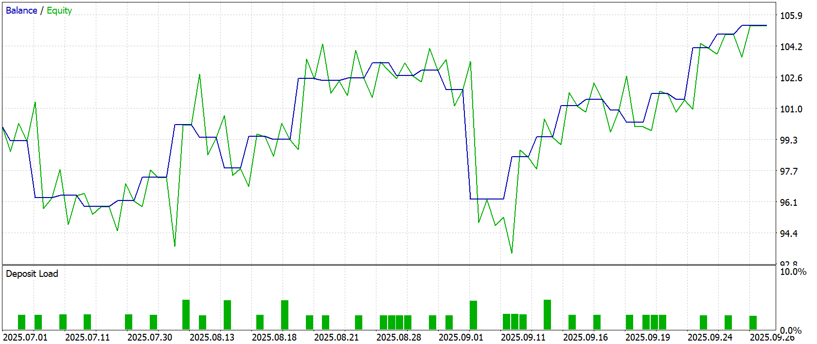
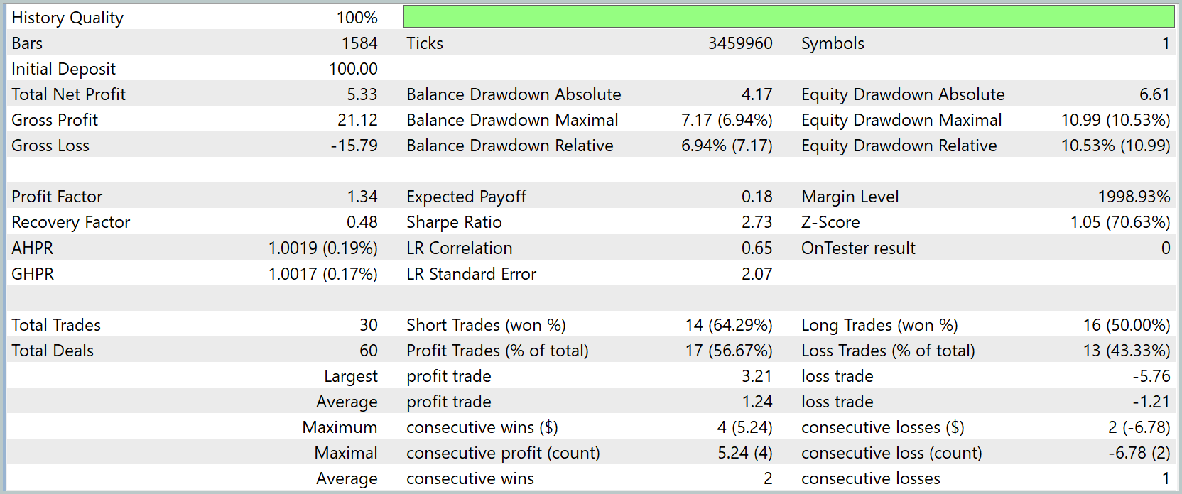
The test results demonstrate the stability and adaptability of the model built using the RAFT framework. The Balance/Equity chart shows that the model is successfully maintaining positive equity growth despite periodic market fluctuations. Both indicators are moving in tandem, which suggests that the model is functioning in a balanced manner and that risk management is adequate.
During testing, with an initial deposit of 100.0 USD, the model generated a net profit of 5.33 USD. The maximum balance drawdown was 7.17%, while the maximum equity drawdown was 10.53%, indicating a reasonably conservative strategy and low risk relative to the amount of capital. The overall profit-to-loss ratio (Profit Factor) is 1.34, confirming a favorable ratio of profits earned to losses incurred.
An analysis of trading operations shows that out of 30 trades executed, 17 were profitable (56.67%). Short positions performed better, with a win rate of 64.29%, compared with a long-position win rate of 50.0%. The average profit per trade is 1.24 USD, and the average loss is 1.21 USD. This demonstrates the balanced nature of the strategy. The largest cumulative profit from consecutive winning trades reached 5.24 USD over 4 trades, while the largest cumulative loss from consecutive losing trades was 6.78 USD over 2 trades.
Overall, the model demonstrates steady positive capital growth, the ability to respond flexibly to changes in market conditions, and effective risk management. RAFT, integrated into the State Encoder, provides an informative representation of market features and enables the system to make informed decisions even in unstable market conditions. However, before using the model in real markets, it is necessary to conduct an additional series of comprehensive strategy tests using a more representative sample.
Conclusion
The RAFT framework has proven to be a powerful tool for analyzing and forecasting financial time series. Its flexible and optimized architecture ensures good forecast accuracy, stable performance, and easy scalability to new tasks. RAFT integrates key components into a single system, accelerating data processing, reducing the risk of errors, and facilitating the creation of effective trading strategies. These advantages make it an indispensable tool for traders and researchers seeking reliable and quick solutions.
Links
Software used in this article
| # | Name | Type | Description |
|---|---|---|---|
| 1 | Study.mq5 | Expert Advisor | Expert Advisor for offline model training |
| 2 | StudyOnline.mq5 | Expert Advisor | Expert Advisor for online model training |
| 3 | Test.mq5 | Expert Advisor | Expert Advisor for model testing |
| 4 | Trajectory.mqh | Class Library | Structure describing the system state and model architectures |
| 5 | NeuroNet.mqh | Class Library | Class library for building a neural network |
| 6 | NeuroNet.cl | Library | Code library for an OpenCL program |
Translated from Russian by MetaQuotes Ltd.
Original article: https://www.mql5.com/ru/articles/20153
Warning: All rights to these materials are reserved by MetaQuotes Ltd. Copying or reprinting of these materials in whole or in part is prohibited.
This article was written by a user of the site and reflects their personal views. MetaQuotes Ltd is not responsible for the accuracy of the information presented, nor for any consequences resulting from the use of the solutions, strategies or recommendations described.

 Building a Prop-Firm Rule Guard in MQL5 (Part 1): The Observation Layer
 Zero-Copy Tick Streaming (Part 2) : Reading MetaTrader 5 Ticks into Python and Benchmarking the Result
 Optimal Trade Exit in MQL5: Longstaff-Schwartz Least-Squares Monte Carlo for Continuation-Value Estimation
 Market Simulation: First Steps with SQL in MQL5 (III)

- Free trading apps
- Over 8,000 signals for copying
- Economic news for exploring financial markets
You agree to website policy and terms of use