Neural Networks in Trading: Iterative Forecast Refinement Models (Key Components)

Introduction

The modern financial market is more than just a collection of quotes and indices. It is a complex, dynamic system in which every price change reflects a whole network of causes, interactions, and expectations. The stream of data arriving every second resembles a living flow in which every moment carries meaning. To see this movement is to learn to read the market as a process, not as a result. This is precisely the goal of the RAFT (Recurrent All-Pairs Field Transforms) framework, whose architecture was originally designed to understand dynamics in image sequences but is also ideally suited to the nature of market time series.

The core concept of the RAFT framework is the ability to think in terms of motion, continuity, and refinement.

In classical trading, price is viewed as a series of discrete values — candlesticks, bars, and ticks. An analyst sees a sequence and tries to identify a pattern. However, the real market flows like a river. It does not jump from point to point, but rather flows from one state to another, changing direction and speed under the influence of a thousand different factors. And this is where the RAFT philosophy becomes particularly clear. The model views the data not as a set of snapshots, but as a stream. Every new state is linked to the previous one by a multitude of hidden dependencies. In computer vision terms, this is optical flow estimation. What matters here is not what is visible in a frame, but how everything moves between frames and in which direction. In financial terms, this is not just a forecast of the next price, but an understanding of the direction and strength of the market's movement.

RAFT is based on the idea of continuously refining the forecast. The model does not reach a final conclusion immediately, but revisits it many times, each time comparing new information with the results already obtained. This recurrent nature is reminiscent of the work of an experienced analyst who adjusts their assumptions as new data becomes available, while maintaining the overall context. As a result, RAFT achieves high stability even amid strong market fluctuations, when traditional algorithms lose synchronization with the stream of events. In financial analysis, this quality is particularly important, since the market is rarely predictable. Impulsive price moves are followed by pullbacks, and even steady trends can sometimes collapse in a matter of minutes. The model's ability to revise its decisions brings it closer to real-world thinking — which is flexible, iterative, and capable of self-adaptation.

From a methodological perspective, the internal structure of RAFT is based on three interrelated ideas:

• feature extraction,
• establishing connections between them,
• iterative refinement of these connections.

Features describe the state of the system. In our case, these are market characteristics: volatility, impulsive price moves, the balance of supply and demand, and correlations between assets. Next, a field of all possible interactions is formed — a sort of market map of connections — in which each point reflects the mutual influence of the system's states over time. Finally, the recurrent block refines this field step by step, bringing the model closer to the most accurate representation of market movements. Thus, RAFT does not simply search for an answer, but rather “engages in a dialogue” with the data, refining its judgments at every step.

At first glance, it might seem that computer vision and financial data have nothing in common. But if we replace frames with time windows and pixels with asset features, it becomes clear just how closely these two worlds are related. In both cases, we are dealing with a stream of information in which each change makes sense only in the context of what came before. Each new tick is not an isolated event, but rather a continuation of the market’s history, woven into the overall fabric of its movement. RAFT creates precisely this context by constructing a displacement field — a sort of map of liquidity movement where one can see the directions and intensity of changes. This opens up possibilities not only for forecasting but also for interpretation. The researcher gains a tool for visualizing market dynamics, capable of identifying where trends are accelerating, where reversals are emerging, and where market forces are reaching equilibrium.

Unlike heavyweight neural network systems, RAFT combines computational efficiency with conceptual depth. Its structure is compact, and the iterative refinement process does not require enormous computational resources. This is particularly valuable for implementation in the MQL5 environment, where code efficiency and data processing speed are top priorities. The model can be adapted to real-world market conditions without compromising its accuracy or stability. Moreover, its recurrent nature makes it possible to respond in real time to a stream of ticks, rather than merely analyzing historical samples.

But perhaps the greatest strength of RAFT is its intellectual flexibility. It does not remain confined to a single pattern or rely on a scheme learned once and for all. Each new snapshot of data prompts the model to reevaluate its own conclusions. This reflects its philosophy — not to predict the market as a static object, but to adapt to its movements and think in tandem with it. In a constantly changing environment, this ability is more valuable than any degree of accuracy: after all, the market is rarely right, but it always remains alive.

In the article, we will focus on the architecture and structure of the RAFT framework. Let's break down how it works and lay the groundwork for implementing it step by step using MQL5. The goal is simple yet ambitious — to demonstrate how this model, designed to analyze motion in video streams, can become a powerful tool for analyzing movements in financial data. After all, if you learn to see structure in this flow, you can get closer to what has always been a trader's dream — understanding where the price is headed and why it is moving in that particular direction.

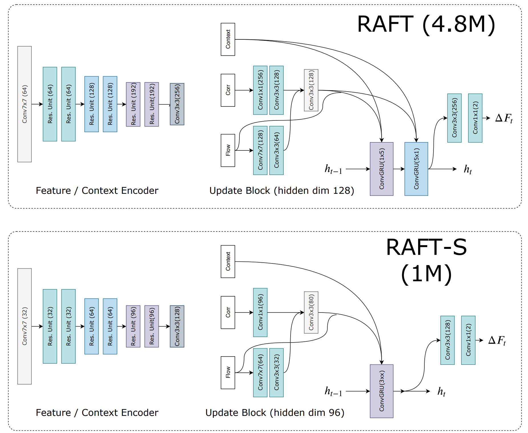
An illustration of the RAFT framework, created by the author, is shown below.

Multiscale Correlation Module

To make the RAFT framework speak the language of the markets, we start by building a feature correlation map. It makes sense to build on the work already done on STE-FlowNet. As before, instead of the fixed initial state proposed by the framework's authors, we use a stack of the system's most recent states. This approach allows the model to see not just the current value of the indicator, but the context of its movement: its dynamics, acceleration, and inertia. It's as if a trader were evaluating not just a single candlestick, but an entire history of price fluctuations, piecing together the cause-and-effect logic behind price behavior.

However, the classical RAFT correlation map is based on a coordinate space in which the displacements of objects have both direction and magnitude. There is no coordinate grid in financial data. Impulsive price moves do not move across features; rather, they evolve over time. Therefore, in our case, scaling is applied along the time axis. We create an analogous correlation pyramid, but along the time axis. Each level reflects a certain history depth — from short-term fluctuations to fundamental trends. This enables RAFT to view the market across multiple time dimensions, capturing both micro-fluctuations and long-term wave structures, thereby forming a more stable and adaptive understanding of the data.

Next, we will set up the creation of a multiscale feature map. First, it is created for each time range, capturing both rapid and slow changes. All of these levels are combined into a single tensor, which is fed into the state stack. This hierarchy enables the model to simultaneously account for both instantaneous market reactions and inertial shifts — aspects that are often overlooked in classical methods.

In the practical section of the previous article, we implemented an OpenCL kernel that aggregates and averages features across all levels of the temporal pyramid. This step made it possible to generate consistent representations of the data at different scales, laying a solid foundation for subsequent calculations. Today, we move on to creating a specialized object for multiscale feature correlation in the main program. It will serve as the core of our implementation of the RAFT mechanism in a financial context — a kind of vision for the system, capable of recognizing relationships between market states with varying history depths.

class CNeuronMultiScaleStackCorrelation :  public CNeuronStackCorrelation
  {
protected:
   uint                 iLevels;
   CNeuronBaseOCL       cScales;
   //---
   virtual bool      AggregationByTime(CNeuronBaseOCL *NeuronOCL);
   virtual bool      AggregationByTimeGrad(CNeuronBaseOCL *NeuronOCL);
   //---
   virtual bool      feedForward(CNeuronBaseOCL *NeuronOCL) override;
   virtual bool      calcInputGradients(CNeuronBaseOCL *NeuronOCL) override;

public:
                     CNeuronMultiScaleStackCorrelation(void) {};
                    ~CNeuronMultiScaleStackCorrelation(void) {};
   //---
   virtual bool      Init(uint numOutputs, uint myIndex, COpenCLMy *open_cl,
                          uint stack_size, uint dimension,
                          uint variables, uint levels,
                          ENUM_OPTIMIZATION optimization_type, uint batch);
   //---
   virtual int       Type(void)   override const   {  return defNeuronMultiScaleStackCorrelation;   }
   //--- Methods for Working with Files
   virtual bool      Save(int const file_handle) override;
   virtual bool      Load(int const file_handle) override;
   //---
   virtual void      SetOpenCL(COpenCLMy *obj) override;
   //---
   virtual uint      GetLevels(void) const { return iLevels; }
   virtual uint      GetVariables(void) override const { return GetVariables() / iLevels; }
  };

The new object inherits the basic functionality of the CNeuronStackCorrelation class and extends the state correlation mechanism by adding support for multiscale analysis — the ability to examine data at multiple levels of temporal depth simultaneously. In the context of financial time series, this is equivalent to monitoring price movements not only in the short term but also on longer time frames.

The structure shown adds a variable, iLevels, that defines the number of scales in the temporal pyramid. In other words, it specifies how many levels of analysis the system will use. Each level corresponds to a specific time window.

The cScales object is an instance of the base class CNeuronBaseOCL and is intended for temporarily storing the feature pyramid of the state being analyzed.

The Init method acts as a kind of architect — it does not just prepare the object for operation, but builds an entire infrastructure for perceiving data at multiple scales. It is here that mathematical logic converges with computational architecture, transforming the abstract idea of a temporal pyramid into a real, functioning mechanism.

bool CNeuronMultiScaleStackCorrelation::Init(uint numOutputs, uint myIndex, COpenCLMy *open_cl,
                                          uint stack_size, uint dimension, uint variables, uint levels,
                                          ENUM_OPTIMIZATION optimization_type, uint batch)
  {
   if(!CNeuronStackCorrelation::Init(numOutputs, myIndex, open_cl, stack_size, dimension,
                                     variables * levels, optimization_type, batch))
      return false;

Calling the method begins the step-by-step initialization of a structure that integrates different analysis time scales into a single system. The following key configuration parameters are passed as input: the number of outputs, the index of the current neuron, a reference to the OpenCL control object, the depth of the time stack, the data dimensionality, the number of features, the number of scales, the optimization type, and the data batch size. Together, all these parameters determine exactly how the neuron will perceive temporal context, how far back into the past it will be able to “look,” and at what level of detail it will analyze the market.

The first step is to call the method of the same name in the parent class. This call can be viewed as laying the foundation. It creates the basic structure of the correlation stack, allocates memory, and prepares OpenCL buffers. But there is one fundamental difference here — the number of features is multiplied by the number of levels in the temporal pyramid. This approach creates a unified feature space in which each level receives its own dataset, reflecting the market over a different time horizon. If the basic initialization fails for any reason, the method immediately terminates execution to avoid unpredictable errors.

After the basic initialization is successfully completed, the number of levels in the temporal pyramid is stored in the variable iLevels. This value serves as an internal reference point for all subsequent calculations and determines how many time scales will be included in the construction of the correlation structure.

   iLevels = levels;
   if(!cScales.Init(0, 0, OpenCL, dimension * levels * variables, optimization, iBatch))
      return false;
//---
   return true;
  }

The next step is to initialize the cScales object, which is responsible for storing multiscale features. Essentially, this is where a digital counterpart to multi-layered perception takes shape: the system begins to view the market simultaneously across several time horizons — from short-term fluctuations to long-term trends.

If the cScales container is created successfully, the method completes the initialization and returns true. This brief but important final step signals that the object is ready for use. From this point on, CNeuronMultiScaleStackCorrelation becomes a full-fledged node in the computational graph, capable of aggregating, scaling, and interpreting the dynamics of financial data over time.

Everything that happens within this method can be thought of as the process of configuring a complex analytical tool, where each parameter has its own meaning and purpose.

The forward pass algorithm in the CNeuronMultiScaleStackCorrelation class implements the core logic of multiscale correlation processing — this is where temporal aggregation, multiscale analysis, and matrix transformations are combined to produce the neural block's final response.

bool CNeuronMultiScaleStackCorrelation::feedForward(CNeuronBaseOCL *NeuronOCL)
  {
   if(!AggregationByTime(NeuronOCL))
      return false;

The method begins by calling the AggregationByTime method, which is a wrapper for the OpenCL kernel of the same name that we implemented in the practical section of the previous article. At this stage, the current features are aggregated along with information about previous states from the stack, organizing them into a logically consistent structure along the time axis. This step makes it possible to identify stable dynamic relationships while simultaneously smoothing out the random fluctuations typical of financial time series.

The next step is to add the resulting information to the stack that stores the state history.

   if(!cStack.FeedForward(cScales.AsObject()))
      return false;

Once all the multiscale components have been computed, the method proceeds to multiply the accumulated history stack by the detailed representation of the state being analyzed. This is where the multiscale features are combined into the final response vector.

   if(!MatMul(cStack.getOutput(), NeuronOCL.getOutput(), Output, GetStackSize() * GetLevels(),
              GetDimension(), 1, GetVariables(), true))
      return false;

Please note that the function's parameters explicitly specify the dimensions of the matrices. A matrix of size [(StackSize × Levels), Dimension] is multiplied by a column vector of size [Dimension]. At the same time, parallel computation of Variables independent products generates correlation matrices for each individual sequence over the given time horizon at the specified number of scales. Essentially, this stage synthesizes information by combining all levels of correlations and scales into a single, generalized result that is ready for further processing.

The final step is to apply the activation function. Of course, if the user has specified one.

   if(activation != None)
      if(!Activation(Output, Output, activation))
         return false;
//---
   return true;
  }

The method's algorithm is structured logically and transparently: from temporal aggregation to multiscale analysis, and then to synthesis and nonlinear response. This architecture makes it possible to effectively extract hidden dependencies from dynamic, multidimensional data while maintaining the structural stability and interpretability of the results.

As you may have noticed, this module does not contain any trainable parameters, but it plays an important role as one of the components of our neural model. And as we know, the model itself requires training. To prevent our multiscale correlation module from hindering training, we must ensure that error gradients are correctly propagated to all nodes in the computational graph according to their contribution to the final result. This mechanism is implemented in the calcInputGradients method.

bool CNeuronMultiScaleStackCorrelation::calcInputGradients(CNeuronBaseOCL *NeuronOCL)
  {
   if(!NeuronOCL)
      return false;

The method begins by verifying that the pointer to the source data object is valid, which helps prevent invalid calls.

The main gradient calculation begins with a call to the MatMulGrad function, which performs a backward pass through matrix multiplication to propagate the error gradients from the output correlation matrices to the original data and the stack of multiscale features.

   if(!MatMulGrad(cStack.getOutput(), cStack.getGradient(),
                  NeuronOCL.getOutput(), cScales.getGradient(),
                  Gradient, GetStackSize()*GetLevels(),
                  GetDimension(), 1, GetVariables(), true))
      return false;

This approach takes into account all levels of the temporal pyramid and every feature, and parallel computation ensures efficient processing of large time series.

Next, AggregationByTimeGrad is called to backpropagate gradients through temporal aggregation. This step ensures that the contribution of each state at a time step is correctly taken into account when adjusting the model parameters.

   if(!AggregationByTimeGrad(NeuronOCL))
      return false;

It is important to note here that the parameters of the state under analysis are involved simultaneously in two processes: matrix multiplication to calculate correlations and the aggregation of multiscale features. Therefore, it is necessary to carefully combine the gradients obtained from these two data streams. The SumAndNormilize function does exactly that. It sums the values, ensuring that the gradients are balanced and consistent. As a result, the model correctly updates its trainable components, preventing the influence of some levels from being overestimated relative to others.

   if(!SumAndNormilize(NeuronOCL.getGradient(), cScales.getGradient(), NeuronOCL.getGradient(),
                                                           GetDimension(), false, 0, 0, 0, 1))
      return false;
   Deactivation(NeuronOCL)
//---
   return true;
  }

The process concludes with a call to Deactivation, which adjusts the gradients using the derivative of the activation function, making them suitable for further propagation.

Ultimately, the calcInputGradients method transforms the multiscale correlation module from a passive component into an active participant in training, carefully distributing the error among all connected components and ensuring stable and correct training of the entire neural model.

2D-GRU Block

Now that we have built the multiscale correlation module, it makes sense to turn our attention to the next critical component — convolutional GRUs. The authors of the RAFT framework propose not one, but two sequential convolutional GRU units. Each of these units operates along a different axis of the coordinate plane. In the visual task, this means that the first group of convolutions can capture horizontal dependencies and the second vertical ones, with their sequential application yielding a deeper representation of local and global displacements. In a financial context, a similar idea is applied along different axes. One GRU branch can model temporal dynamics within a single set of features, while the other can capture interactions between sets of features. The key requirement here is not simply to connect two existing modules in series, but to establish a unified data flow in which hidden states and input data are used together and in sync.

If we try to stitch together two standard implementations in series, we will run into a limitation. Each of them will operate in its own state space and will be unable to effectively share hidden state with a neighboring branch or access the same correlation data simultaneously. We need a module that internally implements two convolutional GRU stages but is treated as a single node within the architecture — with shared interfaces, unified memory management, and a predictable protocol for passing hidden states. Such a module must accept aggregated correlation maps and features as input, have internal buffers for the hidden states of the two stages, and be capable of providing parallel access for both stages to the input tensors without redundant copying.

We implement the concept of two-dimensional data processing proposed by the authors of the RAFT framework in the CNeuronSpikeConvGRU2D class — an extended version of the convolutional GRU, specifically adapted for analyzing signals in two directions. This module inherits the basic functionality from CNeuronSpikeConvGRU but extends it with a second level of computation. This makes it possible to simultaneously account for temporal dependencies and relationships between features. This structure enables a deeper understanding of the data: at each step, the model draws on both the previous state and the spatial context, improving the accuracy of iterative forecast refinement.

class CNeuronSpikeConvGRU2D  :  public CNeuronSpikeConvGRU
  {
protected:
   CNeuronConvOCL       cProjectionX;
   CNeuronBaseOCL       cConcatenated2[2];
   CNeuronConvOCL       cZR2;
   CNeuronBaseOCL       cZ2;
   CNeuronBaseOCL       cR2;
   CNeuronConvOCL       cHt2;
   CNeuronBaseOCL       cH2;
   CNeuronTransposeOCL  cTranspose[3];
   //---
   virtual bool      feedForward(CNeuronBaseOCL *NeuronOCL) override;
   virtual bool      updateInputWeights(CNeuronBaseOCL *NeuronOCL) override;
   virtual bool      calcInputGradients(CNeuronBaseOCL *NeuronOCL) override;

public:
                     CNeuronSpikeConvGRU2D(void) {};
                    ~CNeuronSpikeConvGRU2D(void) {};
   //---
   virtual bool      Init(uint numOutputs, uint myIndex, COpenCLMy *open_cl,
                          uint units, uint chanels_in, uint chanels_out,
                          ENUM_OPTIMIZATION optimization_type, uint batch);
   //---
   virtual int       Type(void)   override const   {  return defNeuronSpikeConvGRU2D;   }
   //--- Methods for Working with Files
   virtual bool      Save(int const file_handle) override;
   virtual bool      Load(int const file_handle) override;
   //---
   virtual void      SetOpenCL(COpenCLMy *obj) override;
   //---
   virtual bool      WeightsUpdate(CNeuronBaseOCL *source, float tau) override;
   //---
   virtual uint      GetChanels(void) const { return cHt.GetFilters(); }
   virtual uint      GetUnits(void) const { return cHt.GetUnits(); }
  };

The main computing nodes are located in the protected section of the class. The cProjectionX component projects the input features into an alternative space, creating an independent representation for the second GRU iteration and aligning the dimensionality of the input features with the hidden-state dimension being analyzed. Essentially, it provides an additional perspective on the data, offering cross-sensitivity between temporal and correlational relationships. This is particularly important in financial analysis, where the behavior of a single asset can affect an entire group of related instruments.

Next come two cConcatenated2[2] buffers, which are used to combine the outputs of the first stage with the input data. This technique creates a richer context in which both new and original features are combined into a single tensor. As a result, the second GRU cell gains a complete picture of the system's state — both the current change and its root cause. This is similar to the process of revising a forecast: first, the model makes a preliminary prediction; then, taking into account the context and refined data, it adjusts its decision.

The cZR2, cZ2, cR2, cHt2, and cH2 blocks make up the internal structure of the second stage of the GRU. Together, they create a closed-loop mechanism with two updates, in which information is refined gradually but continuously.

The three cTranspose[3] objects facilitate data reorientation between stages. From a financial perspective, this allows the model to alternate between the temporal and factor dimensions: viewing the same features either as dynamics over time or as relationships between assets. This adds a multidimensional perspective to the model's understanding of the market, making the analysis spatial rather than linear.

The process of initializing a module's internal components is a carefully planned stage in which each element is assigned its place and functional role within the overall structure. It all starts with a call to the method of the same name in the parent class, which lays the groundwork for the architecture by inheriting the key properties of the classic convolutional GRU.

bool CNeuronSpikeConvGRU2D::Init(uint numOutputs, uint myIndex, COpenCLMy *open_cl,
                                 uint units, uint chanels_in, uint chanels_out,
                                 ENUM_OPTIMIZATION optimization_type, uint batch)
  {
   if(!CNeuronSpikeConvGRU::Init(numOutputs, myIndex, open_cl, units, chanels_in,
                                           chanels_out, optimization_type, batch))
      return false;

This step is not just a formality: it ensures that the OpenCL computing environment is configured correctly, binds the object to the execution context, and creates the basic data structures upon which all subsequent logic is built.

After the base level has been successfully initialized, the cProjectionX block, which performs a projection transformation, is activated. Its purpose is to adapt the input tensors to the model's internal dimensions — that is, to standardize the number of channels and the size of the filters. Essentially, this layer acts as an input bridge that smooths out differences between data scales and prepares the data for deep processing. The activation function for this layer is intentionally disabled — at this stage, the original feature structure must be preserved without introducing additional distortion.

   uint index = 0;
   if(!cProjectionX.Init(0, index, OpenCL, chanels_in, chanels_in, chanels_out, units, optimization, iBatch))
      return false;
   cProjectionX.SetActivationFunction(None);

Next, two cConcatenated2 objects are initialized, each of which is responsible for combining data from different sources. The lack of activation here is no accident — the combination must be linear so as not to disrupt the balance of signals between the model's branches.

   index++;
   for(uint i = 0; i < cConcatenated2.Size(); i++)
     {
      if(!cConcatenated2[i].Init(0, index, OpenCL, 2 * units * chanels_in, optimization, iBatch))
         return false;
      cConcatenated[i].SetActivationFunction(None);
      index++;
     }

The next step is to set up the cTranspose transposition blocks. There are three of them, and each performs a strictly defined function: the first projects the hidden state data from the previous step; the second performs a similar projection of the input data; and the third restores the original structure when passing the new hidden state to the next level. These operations can be compared to flipping a chessboard — the orientation of the data changes, but its logical relationships remain the same. This technique allows the model to process information simultaneously in two dimensions, which is the key feature of the RAFT approach.

   if(!cTranspose[0].Init(0, index, OpenCL, units, chanels_out, optimization, iBatch))
      return false;
   index++;
   if(!cTranspose[1].Init(0, index, OpenCL, units, chanels_out, optimization, iBatch))
      return false;
   index++;
   if(!cTranspose[2].Init(0, index, OpenCL, chanels_out, units, optimization, iBatch))
      return false;

Next, construction begins on the second GRU level, represented by the objects cZR2, cZ2, cR2, and cHt2. The cZR2 component generates a vector for the update and reset gates, which control how much of the previous information is retained and how much is replaced with new data. Its sigmoid activation makes the model's decision-making process smooth and differentiable, which is particularly important for proper training.

   index++;
   if(!cZR2.Init(0, index, OpenCL, 2 * units, 2 * units, 2 * units, chanels_out, 1, optimization, iBatch))
      return false;
   cZR2.SetActivationFunction(SIGMOID);

The cZ2 and cR2 blocks isolate the control signals and prepare them for the next stage — calculating candidates for the new state in cHt2. Here, the TANH activation function is used to provide a balanced range of values and ensure stability during training, even on long time series.

   index++;
   if(!cZ2.Init(0, index, OpenCL, cZR2.Neurons() / 2, optimization, iBatch))
      return false;
   cZ2.SetActivationFunction((ENUM_ACTIVATION)cZR2.Activation());
   index++;
   if(!cR2.Init(0, index, OpenCL, cZR2.Neurons() / 2, optimization, iBatch))
      return false;
   cR2.SetActivationFunction((ENUM_ACTIVATION)cZR2.Activation());
   index++;
   if(!cHt2.Init(0, index, OpenCL, 2 * units, 2 * units, units, chanels_out, 1, optimization, iBatch))
      return false;
   cHt2.SetActivationFunction(TANH);

This entire chain is like a precision timepiece, where each gear is responsible for its own segment of the movement, but together they create a harmonious rhythm.

The final element of the initialization process is cH2, which accumulates the results of data processing. This block brings together all intermediate calculations to create a coherent representation of the system's current state. At this stage, the model is ready to receive a data stream and perform multidimensional analysis, revealing relationships that are not accessible to traditional one-dimensional architectures.

   index++;
   if(!cH2.Init(0, index, OpenCL, units * chanels_out, optimization, iBatch))
      return false;
//---
   return true;
  }

Thus, the Init method builds an entire computational ecosystem in which each component knows exactly where it belongs and interacts with others through a coordinated exchange of information.

The forward-pass algorithm, implemented in the feedForward method, is a carefully structured sequence of computations in which two-dimensional recurrent logic is combined with the principles of convolutional data processing. Each step here is not merely an operation, but a link in a chain of transformations aimed at extracting and synthesizing the deep interrelationships between the spatial and temporal components of the input stream.

bool CNeuronSpikeConvGRU2D::feedForward(CNeuronBaseOCL *NeuronOCL)
  {
   if(!cProjectionX.FeedForward(NeuronOCL))
      return false;
   if(!cTranspose[0].FeedForward(cH.AsObject()))
      return false;
   if(!cTranspose[1].FeedForward(cProjectionX.AsObject()))
      return false;

The algorithm begins by applying a projection transformation to the input data using the cProjectionX block. This element acts as an adapter between the original features and the model's internal representations, converting the data into a format suitable for two-dimensional analysis. Next, the transpose layers — cTranspose[0] and cTranspose[1] — come into play, rearranging the tensors along the coordinate axes. This makes it possible to combine spatial and temporal dimensions, creating a foundation for cross-directional data interaction.

After the data has been preprocessed, the key parameters are calculated: the number of time steps (units), the number of hidden channels (hidden), and the size of the input window (inputs). These parameters define the architectural configuration for the current forward-pass iteration and ensure consistency across all subsequent operations.

   uint units = cHt.GetUnits();
   uint hidden = cHt.GetFilters();
   uint inputs = cHt.GetWindow() - hidden;

Next, the first stage of combining data streams takes place — the Concat operation, which establishes a common context for computing the control gates of the second GRU block. This is where the outputs of the transpose layers are combined.

   if(!Concat(cTranspose[0].getOutput(), cTranspose[1].getOutput(),
              cConcatenated2[0].getOutput(), units, units, hidden))
      return false;

The resulting tensor is passed to the cZR2 block, which is responsible for generating update and reset vectors. These control signals act as neural levers, regulating which parts of past information are retained and which are replaced by new information.

   if(!cZR2.FeedForward(cConcatenated2[0].AsObject()))
      return false;
   if(!DeConcat(cZ2.getOutput(), cR2.getOutput(), cZR2.getOutput(), units, units, hidden))
      return false;

The data are then split into two streams: cZ2 and cR2, each of which performs its own function in the adaptive memory mechanism. The reset stream (cR2) interacts with the output of the first transposed layer, adjusting the degree of influence of the previous state.

   if(!ElementMult(cR2.getOutput(), cTranspose[0].getOutput(), cR2.getPrevOutput()))
      return false;
   if(!Concat(cR2.getPrevOutput(), cTranspose[1].getOutput(), cConcatenated2[1].getOutput(), units, units, hidden))
      return false;
   if(!cHt2.FeedForward(cConcatenated2[1].AsObject()))
      return false;

The results are combined again using a second Concat operation, forming the basis for calculating a new state candidate in the cHt2 block. At this stage, a nonlinear transformation using the TANH activation function takes place, generating an updated representation of the features.

Next, the GateElementMult operation is performed, in which the candidate state cHt2 is mixed with the previous state under the control of the update gate cZ2. This allows the system to dynamically adjust the balance between memory and updating, creating a stable yet flexible internal representation.

   if(!GateElementMult(cHt2.getOutput(), cTranspose[0].getOutput(), cZ2.getOutput(), cH2.getOutput()))
      return false;
   if(!cTranspose[2].FeedForward(cH2.AsObject()))
      return false;

The result is transformed back using cTranspose[2], returning to the original dimension, where the second stage of GRU processing takes place — this time in the conventional direction, as in a standard convolutional GRU.

   if(!Concat(NeuronOCL.getOutput(), cTranspose[2].getOutput(), cConcatenated[0].getOutput(), inputs, hidden, units))
      return false;
   if(!cZR.FeedForward(cConcatenated[0].AsObject()))
      return false;
   if(!DeConcat(cZ.getOutput(), cR.getOutput(), cZR.getOutput(), hidden, hidden, units))
      return false;
   if(!ElementMult(cR.getOutput(), cTranspose[2].getOutput(), cR.getPrevOutput()))
      return false;
   if(!Concat(NeuronOCL.getOutput(), cR.getPrevOutput(), cConcatenated[1].getOutput(), inputs, hidden, units))
      return false;
   if(!cHt.FeedForward(cConcatenated[1].AsObject()))
      return false;
   if(!GateElementMult(cHt.getOutput(), cTranspose[2].getOutput(), cZ.getOutput(), cH.getOutput()))
      return false;

The output then passes through the cNorm normalization block, where the values are stabilized to eliminate accumulated deviations, and is fed to the final stage — the CNeuronSpikeActivation activation function — which gives the model's output a nonlinear response consistent with spiking neural dynamics.

As a result, the entire forward pass algorithm generates a coordinated flow of computations in which each level complements the others, enabling the model to identify multidimensional relationships in the data. This is not merely a sequence of operations, but a kind of dialogue between space and time, in which signals exchange information, refine one another, and reinforce one another. It is precisely this architectural harmony that makes the CNeuronSpikeConvGRU2D module a key component in the implementation of RAFT, providing deep insight into the structure of the data and high adaptability when analyzing complex dynamic processes — from image streams to financial time series.

Today we accomplished substantial, productive work: we built the core components of the RAFT framework, laying the foundation for its computational architecture. It is time to take a short break and let your thoughts settle. The final step lies ahead of us — combining all the modules we have created into a single, coordinated structure. That is exactly what we will focus on in our next article.

Conclusion

In this article, we moved step by step toward a practical implementation of the key ideas of the RAFT framework, adapting them to the specific requirements of financial analysis. We developed a multiscale feature correlation module and implemented a two-dimensional convolutional GRU block that allows us to account for both temporal and structural dependencies in the data. These components represented a logical extension of previous developments and paved the way for the creation of a comprehensive, iterative model for forecasting market dynamics. In the next article, we will integrate all the elements we have created into a single system, test it in practice, and evaluate the effectiveness of the approaches we have implemented using real historical data.

Links

• RAFT: Recurrent All-Pairs Field Transforms for Optical Flow
• Other articles in this series

Files used in the article

#	Name	Type	Description
1	Study.mq5	Expert Advisor	Expert Advisor for offline model training
2	StudyOnline.mq5	Expert Advisor	Expert Advisor for online model training
3	Test.mq5	Expert Advisor	Expert Advisor for model testing
4	Trajectory.mqh	Class Library	Structure describing the system state and model architectures
5	NeuroNet.mqh	Class Library	Class library for building a neural network
6	NeuroNet.cl	Library	Code library for an OpenCL program