

Self-Optimizing Expert Advisors in MQL5 (Part 20): Causality Regularization With Time-Lagged Independent Components Analysis (3)
 178
 0

Introduction
This article addresses the problems faced by practitioners attempting to suppress noise in financial market data while preserving useful information to empower their trading decisions. Distinguishing market noise from a true signal is a materially challenging task; failing to address this problem meaningfully can result in unreliable trading strategies that lose investors' capital and confidence.
Our current time-lagged ICA solution learns to approximate the independent component manifold from financial market data and uses these approximations to forecast a manually defined surrogate target. Below, we shall outline two potential blind spots associated with our current solution:
- The quality of our forecast is implicitly determined by the characteristics of the hand-crafted target we implemented. This makes it difficult to discern if we have obtained the best performance possible. Should algorithmic traders have to toil indefinitely, generating thousands of hand-crafted targets to be confident in their current performance levels?
- The geometric distance between the current ICA manifold and future smoothed returns could be vastly greater than the distance between the future ICA manifold and future smoothed returns. Our current approach may place an unnecessary strain on the model by forcing the model to bridge a large mathematical gap. Alleviating this geometric gap may enhance model reliability.
In concrete terms, we will show that the ICA algorithm can be seen as a valuable coordinate transformation that allows us to forecast in a possibly richer, low-dimensional space that may have less noise than the direct approach of forecasting returns immediately from the approximate ICA manifold. This layered piecewise approach has practical benefits for algorithmic traders:
- In machine learning, you must validate that the target is a function of the observations. Because the ICA manifold is directly constructed from observed price levels, the relationship our models are learning might be better exposed, which in turn may result in improved performance.
- Using the ICA algorithm as its own target generator creates a feedback loop that has the potential to better align our manifold model and the two forecasting models.
After learning to reconstruct future smoothed returns from forecasted independent components, we then had to address the challenge of understanding the relationship between our algorithmic surrogate targets and the smoothed market returns we intended to forecast. To achieve this we explored two possible solutions:
- Learn the average effect brought about by the independent component that grew the most.
- Employ Shapley Additive Explanations to learn how changes in the components affect the target.
These two approaches gave us a balanced picture of the relative importance of each component and the market regimes associated with growth in these components. We compiled these statistics to render refined noise signals that look for regime switches, misaligned trade entries, and disagreements between the average effect of the dominant independent component and the expected effect of our current spectral cluster.
Getting Started in MQL5
To get started with our analysis, we will first write a handy script to fetch the historical data we need for our analysis. This script has been used extensively in all our discussions so far and will be familiar for our returning readers. However, for any new readers joining our discussion, we will give a brief outline of the functionality of the script.
The script accepts important user settings that configure the number of historical bars fetched and the period and mode of the moving average indicator used. The script then fetches the corresponding market data and its historical 5-day lag. These lags are copied for both raw prices and for the technical indicator. This produces a large matrix with 49 columns and as many rows as you specified.
Once you have created the script, drag and drop it onto your symbol of choice with your intended time frame already selected. For our discussion, we will employ the EURUSD pair on the daily time frame.
//+------------------------------------------------------------------+
//|                                                  ICA Filtering   |
//|                                      Copyright 2026, CompanyName |
//|                                       http://www.companyname.net |
//+------------------------------------------------------------------+
#property copyright "Copyright 2024, MetaQuotes Ltd."
#property link      "https://www.mql5.com"
#property version   "1.00"
#property script_show_inputs

//+------------------------------------------------------------------+
//| Global variables                                                 |
//+------------------------------------------------------------------+
int lags = 5;

//+------------------------------------------------------------------+
//| Inputs                                                           |
//+------------------------------------------------------------------+

input group "File Properties"
input(name="Number of Bars") int size = 10;

input group "Technical Indicators"
input(name="MA Period") int MA_PERIOD = 1;
input(name="MA Type") ENUM_MA_METHOD MA_TYPE = MODE_EMA;

//--- File name
string selected_period = (string) MA_PERIOD;
string selected_ma_type = EnumToString(MA_TYPE);

string file_name = Symbol()+ " " + selected_period + " Period " + selected_ma_type + " Noise Filter.csv";

//--- Technical indicators
int      ma_h,ma_l,ma_o,ma_c,file_handle;
double   ma_h_reading[],ma_l_reading[],ma_o_reading[],ma_c_reading[];

//+------------------------------------------------------------------+
//| Our script execution                                             |
//+------------------------------------------------------------------+
void OnStart()
  {

//--- Initialize inidcators
   ma_h = iMA(Symbol(),PERIOD_CURRENT,MA_PERIOD,0,MA_TYPE,PRICE_HIGH);
   ma_l = iMA(Symbol(),PERIOD_CURRENT,MA_PERIOD,0,MA_TYPE,PRICE_LOW);
   ma_o = iMA(Symbol(),PERIOD_CURRENT,MA_PERIOD,0,MA_TYPE,PRICE_OPEN);
   ma_c = iMA(Symbol(),PERIOD_CURRENT,MA_PERIOD,0,MA_TYPE,PRICE_CLOSE);

   if(ma_h == INVALID_HANDLE || ma_l == INVALID_HANDLE ||ma_o == INVALID_HANDLE ||ma_c == INVALID_HANDLE)
     {
      //--- We failed to load the indicators
      Comment("Failed to load Technical Indicators: ",GetLastError());
      return;
     }

   else
     {
      //---Write to file
      file_handle=FileOpen(file_name,FILE_WRITE|FILE_ANSI|FILE_CSV,",");

      for(int i=size+1;i>=1;i--)
        {

         //--- Update indicator values

         //--- High MA
         CopyBuffer(ma_h,0,i,lags+1,ma_h_reading);
         ArraySetAsSeries(ma_h_reading,true);

         //--- Open MA
         CopyBuffer(ma_o,0,i,lags+1,ma_o_reading);
         ArraySetAsSeries(ma_o_reading,true);

         //--- Low MA
         CopyBuffer(ma_l,0,i,lags+1,ma_l_reading);
         ArraySetAsSeries(ma_l_reading,true);

         //--- Close MA
         CopyBuffer(ma_c,0,i,lags+1,ma_c_reading);
         ArraySetAsSeries(ma_c_reading,true);

         //--- Fill in the column names
         if(i == size+1)
           {
            FileWrite(file_handle,
                      //--- Time
                      "Time",
                      //--- OHLC
                      "Open",
                      "High",
                      "Low",
                      "Close",
                      //--- OHLC Lag 1
                      "Open Lag 1",
                      "High Lag 1",
                      "Low Lag 1",
                      "Close Lag 1",
                      //--- OHLC Lag 2
                      "Open Lag 2",
                      "High Lag 2",
                      "Low Lag 2",
                      "Close Lag 2",
                      //--- OHLC Lag 3
                      "Open Lag 3",
                      "High Lag 3",
                      "Low Lag 3",
                      "Close Lag 3",
                      //--- OHLC Lag 4
                      "Open Lag 4",
                      "High Lag 4",
                      "Low Lag 4",
                      "Close Lag 4",
                      //--- OHLC Lag 5
                      "Open Lag 5",
                      "High Lag 5",
                      "Low Lag 5",
                      "Close Lag 5",
                      //--- Indicators
                      "MA O",
                      "MA H",
                      "MA L",
                      "MA C",
                      //--- Indicators lag 1
                      "MA O Lag 1",
                      "MA H Lag 1",
                      "MA L Lag 1",
                      "MA C Lag 1",
                      //--- Indicators lag 2
                      "MA O Lag 2",
                      "MA H Lag 2",
                      "MA L Lag 2",
                      "MA C Lag 2",
                      //--- Indicators lag 3
                      "MA O Lag 3",
                      "MA H Lag 3",
                      "MA L Lag 3",
                      "MA C Lag 3",
                      //--- Indicators lag 4
                      "MA O Lag 4",
                      "MA H Lag 4",
                      "MA L Lag 4",
                      "MA C Lag 4",
                      //--- Indicators lag 5
                      "MA O Lag 5",
                      "MA H Lag 5",
                      "MA L Lag 5",
                      "MA C Lag 5"
                     );
           }

         //--- Fill in the column values
         else
           {
            FileWrite(file_handle,
                      iTime(_Symbol,PERIOD_CURRENT,i),
                      //--- OHLC
                      iOpen(_Symbol,PERIOD_CURRENT,i),
                      iHigh(_Symbol,PERIOD_CURRENT,i),
                      iLow(_Symbol,PERIOD_CURRENT,i),
                      iClose(_Symbol,PERIOD_CURRENT,i),
                      //--- OHLC Lag 1
                      iOpen(_Symbol,PERIOD_CURRENT,i+1),
                      iHigh(_Symbol,PERIOD_CURRENT,i+1),
                      iLow(_Symbol,PERIOD_CURRENT,i+1),
                      iClose(_Symbol,PERIOD_CURRENT,i+1),
                      //--- OHLC Lag 2
                      iOpen(_Symbol,PERIOD_CURRENT,i+2),
                      iHigh(_Symbol,PERIOD_CURRENT,i+2),
                      iLow(_Symbol,PERIOD_CURRENT,i+2),
                      iClose(_Symbol,PERIOD_CURRENT,i+2),
                      //--- OHLC Lag 3
                      iOpen(_Symbol,PERIOD_CURRENT,i+3),
                      iHigh(_Symbol,PERIOD_CURRENT,i+3),
                      iLow(_Symbol,PERIOD_CURRENT,i+3),
                      iClose(_Symbol,PERIOD_CURRENT,i+3),
                      //--- OHLC Lag 4
                      iOpen(_Symbol,PERIOD_CURRENT,i+4),
                      iHigh(_Symbol,PERIOD_CURRENT,i+4),
                      iLow(_Symbol,PERIOD_CURRENT,i+4),
                      iClose(_Symbol,PERIOD_CURRENT,i+4),
                      //--- OHLC Lag 5
                      iOpen(_Symbol,PERIOD_CURRENT,i+5),
                      iHigh(_Symbol,PERIOD_CURRENT,i+5),
                      iLow(_Symbol,PERIOD_CURRENT,i+5),
                      iClose(_Symbol,PERIOD_CURRENT,i+5),
                      //--- Indicators
                      ma_o_reading[0],
                      ma_h_reading[0],
                      ma_l_reading[0],
                      ma_c_reading[0],
                      //--- Indicators lag 1
                      ma_o_reading[1],
                      ma_h_reading[1],
                      ma_l_reading[1],
                      ma_c_reading[1],
                      //--- Indicators lag 2
                      ma_o_reading[2],
                      ma_h_reading[2],
                      ma_l_reading[2],
                      ma_c_reading[2],
                      //--- Indicators lag 3
                      ma_o_reading[3],
                      ma_h_reading[3],
                      ma_l_reading[3],
                      ma_c_reading[3],
                      //--- Indicators lag 4
                      ma_o_reading[4],
                      ma_h_reading[4],
                      ma_l_reading[4],
                      ma_c_reading[4],
                     //--- Indicators lag 5
                      ma_o_reading[5],
                      ma_h_reading[5],
                      ma_l_reading[5],
                      ma_c_reading[5]
                     );
           }
        }

     }
//--- Close the file
   FileClose(file_handle);
  }
//+------------------------------------------------------------------+
Analyzing Our Market Data in Python
We can now start analyzing our historical market data. Our goal here is to demonstrate that the future growth in the ICA manifold can be forecasted with higher accuracy than our current surrogate target. We will compare our accuracy in classifying changes in smoothed returns against our ability to classify changes in the ICA manifold and empirically observe changes in performance. First, import the libraries we need for general tasks.
#Load standard libraries
import pandas as pd
import numpy as np
import matplotlib.pyplot as plt
import seaborn as sns
Now, read in the data.
data = pd.read_csv("./EURUSD Noise Filter.csv") Fetch the statistical libraries we need. The FastICA algorithm will be used to learn a better representation of our dataset and to create new surrogate targets that we can forecast with impressive accuracy. Spectral clustering is a powerful clustering algorithm that can handle non-convex sets. This means it can still find meaningful clusters even if our dataset is not that well separated and clusters overlap.
#Load FastICA
from sklearn.decomposition import FastICA
#Spectral Clustering
from sklearn.cluster import SpectralClustering
#One hot encoding
from sklearn.preprocessing import OneHotEncoder as OHE
Group our inputs so that we can easily focus on the technical indicator values.
#Group the inputs
OHLC = data.iloc[:,1:25].columns
MA   = data.iloc[:,25:49].columns
ALL  = data.iloc[:,1:].columns
Label the data and manually create a surrogate target.
#Define our forecast horizon
HORIZON = 5

#Label the data with a real valued target
data['C Target']   = data['Close'].shift(-HORIZON) - data['Close']
data['New Target'] = data['MA C'].shift(-HORIZON) - data['MA C']

#Label the data with a binary target
data['C Bin Target']   = 0
data['New Bin Target'] = 0

data.loc[data['C Target'] > 0,'C Bin Target'] = 1
data.loc[data['New Target'] > 0,'New Bin Target'] = 1
Drop missing rows from our matrix.
#Filter missing rows
data = data.iloc[:-HORIZON,:]
Partition our dataset into a training and test set. We will not fit our model on the test set.
#Train test split
train , test = data.iloc[:(-365*3),:] , data.iloc[(-365*3):,:]
Let us now prepare our ICA manifold.
#Prepare our FastICA encoder
enc = FastICA(random_state=0,whiten_solver='eigh',whiten='unit-variance',tol=0.21544346900318778,n_components=8,fun='cube',algorithm='parallel')

#Names of our manifold columns
columns = []
col_name = 'Manifold '
for i in np.arange(8):
    addition = col_name + str(i+1)
    columns.append(addition)

manifold = pd.DataFrame(enc.fit_transform(train.loc[:,MA]),columns=columns)
Join the ICA manifold to the rest of the training set.
train = train.join(manifold)
Create a new group of inputs to mark the manifold columns.
MANIFOLD = train.iloc[:,-8:].columns
MANIFOLD
Index(['Manifold 1', 'Manifold 2', 'Manifold 3', 'Manifold 4', 'Manifold 5','Manifold 6', 'Manifold 7', 'Manifold 8'],dtype='object')
Forecasting Independent Components
Let us now assess our accuracy in forecasting each independent component. Because our initial surrogate target and our new candidates exist on different scales, RMSE may be a misleading comparison metric. Therefore, we will instead represent the growth in each component as a binary target to ensure meaningful comparisons can be made.
#Let us assess our accuracy forecasting each independent component
for i in np.arange(8):
    #The name of the independent component we are currently working with
    input_col = 'Manifold ' + str(i+1)
    #The binary target we are creating for this component
    target_col = 'Manifold Target '+str(i+1)
    train[target_col] = 0
    #Label the growth in each independent component
    train.loc[train[input_col].shift(-HORIZON) > train[input_col],target_col] = 1
Before reviewing the results, verify that the matrix is well-defined. A simple check is each column's mean: values near 0 or 1 indicate sparsity or imbalance. Here, the means are near 0.5, so the matrix is dense and has a balanced mix of 0s and 1s.
#Inspect each target mean
train.iloc[:,-8:].mean()
| Surrogate Target | Target Mean |
|---|---|
| Manifold Target 1 | 0.491325 |
| Manifold Target 2 | 0.503980 |
| Manifold Target 3 | 0.501327 |
| Manifold Target 4 | 0.497857 |
| Manifold Target 5 | 0.498469 |
| Manifold Target 6 | 0.472954 |
| Manifold Target 7 | 0.522352 |
| Manifold Target 8 | 0.492549 |
Calculate the growth in each independent component and store it in the training set. Also, filter out the last batch of rows from the training set where we could not calculate the growth in the manifold on the training set.
#Calculate the growth in each independent component
train.loc[:,MANIFOLD] = train.loc[:,MANIFOLD].shift(-HORIZON) - train.loc[:,MANIFOLD]

#Filter any missing rows
train = train.iloc[:-HORIZON,:]
manifold = manifold.iloc[:-HORIZON,:]
We will now create a new column to denote which independent component has grown the most over our forecast horizon. This is simply calculated as the argmax of the manifold group from our training set. Note that we are not interested in the largest value but the column that contains the largest value. Setting the axis parameter to 1 means that we are performing this check on each row of our training set.
#We will store which component has grown the most
train['State'] = 0

#Keep track of which component grew the most
train['State'] = np.argmax(np.abs(train.loc[:,MANIFOLD]),axis=1)
Naturally, we may want to know which component tends to grow the most across our entire training period. This question can be readily answered by a histogram taken on the state vector of our training set. Our histogram reveals that components 2 and 6 tend to dominate our forecasts almost half of the time. With component 5 dominating the least.
sns.histplot(data=train,x='State',hue='State',bins=24,palette='bright')
The Dominance of Each Independent Component Across Our Training Set
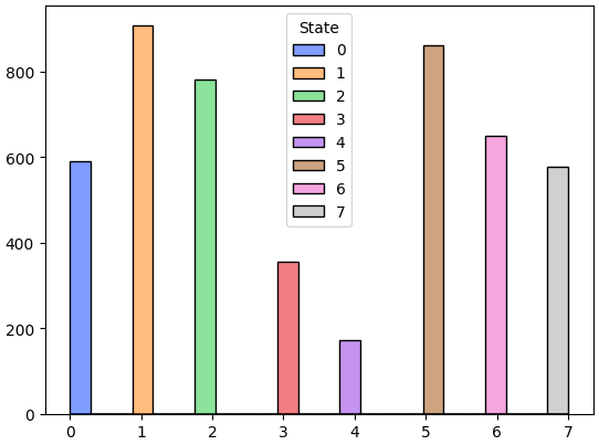
Figure 1: Given the few number of observations that belong to component 5, we may want to interpret its associated statistics carefully.
Let us now learn the average effect brought about as each component dominates the manifold growth. We would like to learn the changes in average return and market risk that can be expected when each component dominates the others.
#Keep track of the average risk and return associated with each dominant component
avg_return = []
avg_risk   = []
for i in np.arange(8):
    avg_return.append(train.loc[train['State'] == i,'C Target'].mean())
    avg_risk.append(train.loc[train['State'] == i,'C Target'].std())
We will first consider how the average return changes across each dominant component. Some components, such as component number 7, have expected returns close to 0. This may indicate to us that when component number 7 grows the most, the market tends to enter a mean-reverting mode. While other components, such as components 2 and 3, appear to be associated with trending market modes, as indicated by their strong returns.
sns.barplot(avg_return,palette='muted')
plt.ylabel('Expected Return')
plt.xlabel('Largest Growing Component')
plt.title('Distribution of Returns Across ICA Components')
The Expected Return Across Each Dominant ICA Component
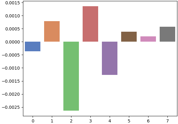
Figure 2: The expected returns associated with each component gives us an idea of the effect the component has on the target.
Market risk appears to spike above average on components 4 and 5. However, if the reader refers back to Figure 1, they will recall that these components only dominated in growth a few times. Therefore, the small number of observations belonging to this group may distort the statistics we are trying to learn.
sns.barplot(avg_risk,palette='muted')
plt.axhline(np.mean(avg_risk),color='red')
plt.ylabel('Market Risk')
plt.xlabel('Largest Growing Component')
plt.title('Distribution of Risk Across ICA Components')
The Distribution of Market Risk Across ICA Components
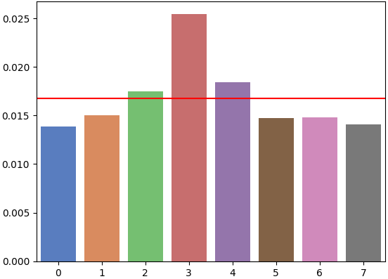
Figure 3: The association of risk varies almost uniformly across each component, with only a few exceptions.
Let us now load the statistical analysis tools we need.
from sklearn.model_selection import TimeSeriesSplit,cross_val_score
from sklearn.discriminant_analysis import LinearDiscriminantAnalysis as LDA
Define our time-series cross-validation object.
tscv = TimeSeriesSplit(n_splits=5,gap=HORIZON) Benchmark our performance forecasting price directly from the ICA manifold. We produced an accuracy of 63%.
old_acc = np.mean(cross_val_score(LDA(),manifold,train.loc[:,'New Bin Target'],cv=tscv,scoring='accuracy'))
old_acc
np.float64(0.6319018404907976)
Now let us record our accuracy forecasting changes in the ICA manifold directly from our lagged market data.
manifold_acc = []

for i in np.arange(8):
    target_col = 'Manifold Target '+str(i+1)
    manifold_acc.append(np.mean(cross_val_score(LDA(),train.loc[:,MA],train.loc[:,target_col],cv=tscv,scoring='accuracy')))
Our average accuracy forecasting changes in the ICA manifold were 76%. This represents an almost 21% improvement in comparison with our ability to forecast the surrogate target we manually defined.
np.mean(manifold_acc) np.float64(0.7653680981595092)
Let us visualize the results we have obtained. We have plotted our accuracy forecasting each independent component as a bar graph. The graph suggests that we are performing exceptionally well at forecasting the first independent component. Our average accuracy over the entire ICA manifold is represented by the solid red line on the graph, while the dotted black line represents our average accuracy forecasting our hand-crafted surrogate target.
sns.barplot(manifold_acc,palette='bright')
plt.axhline(np.mean(manifold_acc),color='red')
plt.axhline(old_acc,color='black',linestyle=':')
plt.title(f'Average Manifold Accuracy: {(np.mean(manifold_acc)*100):.2f}%')
Visualizing Our Accuracy in Forecasting Each Independent Component
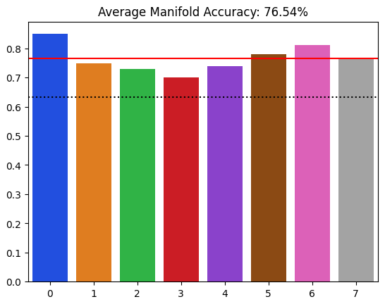
Figure 4: We can forecast the growth in the ICA manifold with greater accuracy than we can forecast smoothed returns.
Now that we have demonstrated that the ICA manifold generates richer surrogate targets than we can manually engineer over the same space of time, let us now observe if our ability to reconstruct future smoothed returns is better than the performance levels we would obtain from the direct approach. We will start by importing the statistical tools we need.
from sklearn.neighbors import KNeighborsRegressor as KNR
from sklearn.model_selection import RandomizedSearchCV
from sklearn.metrics import root_mean_squared_error as RMSE
To ensure a fair comparison, we will tune all the models we are interested in. We have 5 models to optimize. The first 3 models are part of our iterative solution. The last 2 models will be used as benchmarks that our chain of models should outperform. The first benchmark captures the results we would have obtained by forecasting smoothed returns using our moving average indicator readings as inputs. The second benchmark reflects the performance we would have reached if we forecasted smoothed returns immediately from approximated ICA components. Each of the 5 models will be allowed 100 optimization iterations over the training set before being evaluated on the out-of-sample test set.
#Initialize the models
#Suggested solution: Chain of models
#The first model approximates 8 ICA manifold from our market data
ica_embeddings_model = KNR(n_jobs=-1)
#The second model forecasts future ICA manifold growth
ica_forecast_model = KNR(n_jobs=-1)
#The last model attempts to reconstruct the original target given forecasted ICA components
returns_reconstruction_model = KNR(n_jobs=-1)

#Control solution: Benchmark models
#This benchmark model will demonstrate the error levels produced by using moving average inputs
benchmark_model = KNR(n_jobs=-1)
#This benchmark model will demonstrate the error levels produced by our previous methodology of forecasting
#smoothe market returns directly from approximated ICA manifold
benchmark_model_2 = KNR(n_jobs=-1)
Let us define the tuning parameters shared by our models.
#Initialize the parameters to be searched
param_distribution = {
'n_neighbors':[5,10,15,20,30,50,90,150],
'weights':['uniform','distance'],
'algorithm':['auto','ball_tree','kd_tree','brute'],
'leaf_size':[10,20,30,40,50,60,70,80]
}
Search for the best possible model we can build to approximate our ICA manifold given the original market data.
#Initialize the random search object
rscv = RandomizedSearchCV(ica_embeddings_model,param_distribution,random_state=0,n_iter=100,cv=tscv,n_jobs=-1,scoring='neg_mean_squared_error')

#Search
results = rscv.fit(train.loc[:,MA],manifold)
Save the best model we found.
ica_embeddings_model = KNR(weights=results.best_params_['weights'],n_neighbors=results.best_params_['n_neighbors'],leaf_size=results.best_params_['leaf_size'],algorithm=results.best_params_['algorithm'])
At this point, the reader should note that our current setup relies heavily on resampling the training set. Each subsequent model is trained over essentially the same data that the previous model was trained on. This may inflate the performance metrics we obtain on the training set. Let us fit the model responsible for approximating our ICA components from raw market data.
#Fit the model
ica_embeddings_model.fit(train.loc[:,MA],manifold)

#Store the model's predictions
ica_predictions = ica_embeddings_model.predict(train.loc[:,MA])
Next, we will optimize the model that learns to forecast the growth in the ICA manifold given current approximated ICA components and store its predictions.
#Initialize the random search object
rscv = RandomizedSearchCV(ica_forecast_model,param_distribution,random_state=0,n_iter=100,cv=tscv,n_jobs=-1,scoring='neg_mean_squared_error')

#Search
results = rscv.fit(ica_predictions,train.loc[:,MANIFOLD])

#Fit the model
ica_forecast_model = KNR(weights=results.best_params_['weights'],n_neighbors=results.best_params_['n_neighbors'],leaf_size=results.best_params_['leaf_size'],algorithm=results.best_params_['algorithm'])
ica_forecast_model.fit(ica_predictions,train.loc[:,MANIFOLD])

#Store forecasted ICA values
ica_forecast = ica_forecast_model.predict(ica_predictions)
Lastly, we are eager to learn to reconstruct the smoothed market return from the growth we expect to observe in the ICA components.
#Learn to reconstruct the target given forecasted ICA components
#Initialize the random search object
rscv = RandomizedSearchCV(returns_reconstruction_model,param_distribution,random_state=0,n_iter=100,cv=tscv,n_jobs=-1,scoring='neg_mean_squared_error')

#Search
results = rscv.fit(ica_forecast,train.loc[:,'New Target'])

#Fit the model
returns_reconstruction_model = KNR(weights=results.best_params_['weights'],n_neighbors=results.best_params_['n_neighbors'],leaf_size=results.best_params_['leaf_size'],algorithm=results.best_params_['algorithm'])
returns_reconstruction_model.fit(ica_forecast,train.loc[:,'New Target'])
Now we will optimize our first benchmark. The reader should recall that this model learns to forecast future smoothed returns directly from the readings of our moving average indicators.
#This benchmark model emulates the results we would obtain by using moving average inputs to forecast smoothed returns
rscv = RandomizedSearchCV(benchmark_model,param_distribution,random_state=0,n_iter=100,cv=tscv,n_jobs=-1,scoring='neg_mean_squared_error')

#Search
results = rscv.fit(train.loc[:,MA],train.loc[:,'New Target'])

#Fit the model
benchmark_model = KNR(weights=results.best_params_['weights'],n_neighbors=results.best_params_['n_neighbors'],leaf_size=results.best_params_['leaf_size'],algorithm=results.best_params_['algorithm'])
benchmark_model.fit(train.loc[:,MA],train['New Target'])
We will also optimize our second benchmark model that learns to forecast smoothed returns from an approximated ICA manifold.
#The second benchmark model emulates the results we would obtain by using approximate ICA embeddings to forecast smoothed returns
rscv = RandomizedSearchCV(benchmark_model_2,param_distribution,random_state=0,n_iter=100,cv=tscv,n_jobs=-1,scoring='neg_mean_squared_error')

#Search
results = rscv.fit(ica_predictions,train.loc[:,'New Target'])

#Fit the model
benchmark_model_2 = KNR(weights=results.best_params_['weights'],n_neighbors=results.best_params_['n_neighbors'],leaf_size=results.best_params_['leaf_size'],algorithm=results.best_params_['algorithm'])
benchmark_model_2.fit(ica_predictions,train['New Target'])
Prepare an array to store the performance of each workflow on out-of-sample test data.
results = []
We will start by recording the performance of the simplest workflow possible, forecasting smoothed returns from our moving average indicator readings.
#Out of sample testing for benchmark 1: Using ordinary technical indicators as inputs
results.append(RMSE(test['New Target'],benchmark_model.predict(test.loc[:,MA])))
Next, we will store our approximated independent components on the test set. The reader should recall that none of the models we are using have been fit on the test set.
#Now store our approximated ICA manifold
ica_predictions_test = ica_embeddings_model.predict(test.loc[:,MA])
We are now ready to record our second performance benchmark. This benchmark reflects the methodology we employed in our previous discussion of time-lagged independent components analysis. In this setup, we forecast smoothed returns directly from the approximated ICA manifold.
#Out of sample testing for benchmark 2: Using approximated ICA manifold to forecast smoothed returns
results.append(RMSE(test['New Target'],benchmark_model_2.predict(ica_predictions_test)))
Lastly, we will record our new performance levels using our piecewise solution. This solution takes an additional step of forecasting the growth in the ICA manifold and then forecasting smoothed market returns from the expected growth in the ICA manifold.
#Our new performance
results.append(RMSE(test['New Target'],returns_reconstruction_model.predict(ica_forecast_model.predict(ica_predictions_test))))
We will now plot our results as a bar plot. We can observe that our proposed solution produced the lowest out-of-sample error rate. The improvement in our error levels is modest but still consistent with our expectations.
sns.barplot(results,palette='bright')
plt.axhline(np.min(results),color='red',linestyle=':')
plt.scatter(np.argmin(results),np.min(results),color='red')
plt.xticks([0,1,2],['Benchmark 1','Benchmark 2','Suggested Solution'])
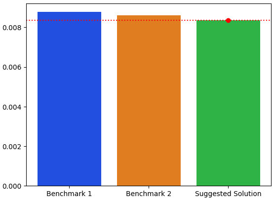
Figure 5: Our out-of-sample test results indicate our piecewise solution was the best performing workflow.
| Methodology | RMSE |
|---|---|
| Benchmark 1: Forecasting smoothed returns directly from moving average indicator readings. | 0.008772881484539027 |
| Benchmark 2: Forecasting smoothed returns directly from an approximated ICA manifold. | 0.00861734614263884 |
| Piecewise approach: Forecasting smoothed returns from the forecasted growth in the ICA manifold. | 0.008358825758359674 |
Understanding How Our Forecasted Components Fit In With Our Strategy
So far, we have demonstrated that the ICA algorithm can be used as an algorithmic generator of rich surrogate targets. We observed that by forecasting the growth in these components, our model can reconstruct the intended target, with greater accuracy than what we were capable of attaining with our previous direct approach. Now, we wish to understand how these forecasted components interact with the rest of our strategy. This task can be broken down into 2 primary objectives:
- Understanding the relative importance of each independent component and the effect that component has on our ability to reconstruct the final target.
- Searching for interactions between our ICA manifold and the spectral clusters we identified in our previous discussion.
Our first task may be answered by Shapley additive explanations (SHAP). Afterward, we will search for interactions and dependencies between our ICA manifold and the spectral clusters in our dataset by building a covariance matrix between the two.
Obtaining SHAP Explanations
SHAP explanations are a mathematically principled tool for understanding the inner workings of a machine learning model. The SHAP algorithm was originally inspired by developments in the mathematical field of game theory. SHAP explanations offer us robust model-agnostic explanations of global and local model behavior. We have covered the SHAP algorithm in detail in our previous discussion on "The Disagreement Problem: Diving Deeper into The Complexity Explainability in AI." For readers who may want a refresher, a link to that article is provided here. To get started, we will import the SHAP library and the surrogate model we wish to explain.
import shap
from sklearn.neighbors import KNeighborsClassifier
Convert the predictions made by the model responsible for approximating our ICA components from a numpy n-dimensional array to a pandas DataFrame.
#Convert our ICA model forecasts into a pandas DataFrame
ica_forecast = pd.DataFrame(ica_forecast_model.predict(ica_predictions),columns=MANIFOLD,index=train.index)
Now fit the model to predict the future smoothed market return, given forecasted ICA components.
explained_model = KNeighborsClassifier()
explained_model.fit(ica_forecast,train['New Bin Target'])
We want to understand our model's behavior over the entire training set. To do this, we will first define a utility function that will return the predicted probabilities our classifier assigns to each training instance. Then we will store the median values of our ICA forecasted components. These median values are used by the SHAP algorithm to compare the effect each component has, in light of the average effect brought about by that component. These median values are then passed to our SHAP explainer, along with the utility function we designed to return the expected probability of price levels rising given the forecasted ICA components. Finally, we pass our SHAP explainer the entire training set to obtain both global and local explanations.
def get_expected_probabilities(x):
    return explained_model.predict_proba(x)[:, 1]

median =ica_forecast.median().values.reshape((1, ica_forecast.shape[1]))

explainer = shap.Explainer(get_expected_probabilities, median)

shap_values = explainer(ica_forecast.iloc[:, :])
Global SHAP explanations help us understand the importance of each feature the model was trained on, whereas local explanations give us a case-by-case breakdown of each prediction our model made and how the input values affected its prediction. Let us first obtain a global explanation of our final model that is responsible for reconstructing the smoothed market return, given forecasted growth across ICA components.
In Figure 6 below, we have made a bee-swarm plot of the global importance of each ICA component. The components are arranged with the most important feature at the top and the least important feature at the bottom. In our case the growth in the second, eighth, and third ICA components was estimated to be the top 3 most important inputs by the SHAP explainer.
It is interesting to note that the models that consistently grew the most in our ICA manifold were not necessarily the most important features identified by the SHAP explainer.
The SHAP explainer also attempts to help us understand what happens to our model's output when each of the inputs is above or below its average. Blue points indicate low feature values, while pink points indicate high feature values. The direction of influence that these extreme values had is represented by the points' position along the x-axis. Data points that pushed the model's output higher are on the right of the x-axis, while points on the left of the x-axis pushed the model's predictions lower.
Generally speaking, most of the points on the right-hand side of the x-axis are blue, while most of the pink points are on the left-hand side. This may suggest that high values in the independent components influence the model to forecast lower returns, and the opposite appears true of low input values.
shap.plots.beeswarm(shap_values) 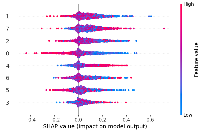
Figure 6: SHAP explanations help us understand the importance of each input we have.
Local explanations can be obtained to help us understand individual predictions made by our model. Waterfall plots help us understand why a particular prediction was made on a selected day; for example, we may want to understand how our model's predictions were being made on the day of an important macroeconomic news announcement. The model's inputs are ordered according to the impact they had on the model's final output. In the example below, we can see that on training instance number 99, most of the model's inputs encouraged a bullish forecast. The model was strongly influenced by components 5 and 1. Armed with the true outcome of the day, we can quickly identify noisy components that may repeatedly give false trading signals around important days.
shap.plots.waterfall(shap_values[98]) 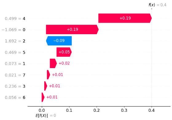
Figure 7: Local explanations help us understand the individual contribution each component made on a particular training day.
Searching for Interactions Between Our Spectral Clusters and the Growth in Our ICA Components
Our trading strategy is growing in complexity. It may be possible that there are rich relationships and interactions unexpectedly taking shape between ICA components we have optimized and the spectral clusters we identified in our previous discussion. If such interactions exist, it would be challenging for us to directly observe these patterns due to the high number of dimensions involved. Fortunately, there exist a myriad of statistical algorithms that allow us to automatically identify relationships in data. One of these algorithms is implemented by calculating a covariance matrix between the two. To do this, we will first reproduce the ideal clustering setup we learned from our previous discussion.
#Reproduce the best clustering setup
cls = SpectralClustering(n_clusters=8,assign_labels='cluster_qr')
ohe = OHE(sparse_output=False)
cls.fit(train.loc[:,MA])
train['Cluster'] = cls.labels_
Create a dedicated matrix to store the cluster labels in a one-hot-encoded form. In this form, only a single column will have the value 1, indicating which cluster we are in, while all remaining columns will have a value of 0.
#Create a dataframe to store our one-hot-encoded cluster labels
clusters = pd.DataFrame(ohe.fit_transform(train[['Cluster']]),columns=['Cluster 1','Cluster 2','Cluster 3','Cluster 4','Cluster 5','Cluster 6','Cluster 7','Cluster 8'])
It is imperative that all our matrices be of the same size. If this is overlooked, the rest of our analysis cannot be completed. Therefore, we encourage you to check if this is true. The train set should have the same number of rows as the remaining 2 matrices. This number may differ from yours depending on how many bars of historical data you fetched and your forecasting horizon.
train.shape
(4894, 62)
The manifold matrix should have the same number of rows as the training matrix and share the same number of columns as the cluster matrix.
manifold.shape
(4894, 8)
As we can see, all 3 matrices have the correct shapes we expect.
clusters.shape
(4894, 8)
Recall, we are keen to learn if there is a relationship between the independent components and the spectral clusters. We can achieve this by calculating a contingency table between the current state of the growth in our components and the cluster we are in. The first step we take is to create a one-hot-encoded matrix that denotes the state of our component growth in a fashion similar to that described for our clustering matrix. Meaning, the column that corresponds to the cluster that grew the most will have a value of one; all other columns will have a value of 0.
#Prepare to create a covariance matrix to learn how our independent components relate with our spectral clusters
ohe = OHE(sparse_output=False)
ica_state = pd.DataFrame(ohe.fit_transform(train[['State']]),columns=['ICA 1','ICA 2','ICA 3','ICA 4','ICA 5','ICA 6','ICA 7','ICA 8'])
Compute the contingency table via matrix multiplication. The order is fine as long as the left matrix is transposed; otherwise, you will produce a 4984×4984 matrix in this setup.
#Prepare to create a conditional frequency heatmap to learn how our independent components relate with our spectral clusters
ohe = OHE(sparse_output=False)
ica_state = pd.DataFrame(ohe.fit_transform(train[['State']]),columns=['ICA 1','ICA 2','ICA 3','ICA 4','ICA 5','ICA 6','ICA 7','ICA 8'])

#Create a conditional frequency matrix between our ICA state and Spectral clusters
ica_sc_con_freq = ica_state.T @ clusters
ica_sc_con_freq
Each row of the resulting contingency table is then scaled to have a sum of 1. This gives us a lot of meaningful information, which can be viewed as a heatmap. We can observe that all our components tend to be most associated with cluster 8. From our previous discussion, we observed that cluster 8 has a positive expected return. We could couple this information with the expected return across each independent cluster to find a trading strategy suited to exploit cluster 8. Unfortunately, this may not be feasible, however, because cluster 8 was the hardest cluster for us to learn from our dataset. Trading strategies exploiting cluster 8 may be very noisy.
for i in np.arange(ica_sc_con_freq.shape[0]):
    ica_sc_con_freq.iloc[i,:] = ica_sc_con_freq.iloc[i,:] / ica_sc_con_freq.iloc[i,:].sum()

sns.heatmap(ica_sc_con_freq,annot=True)
The Contingency Table Calculated Between Our Independent Components and Spectral Clusters
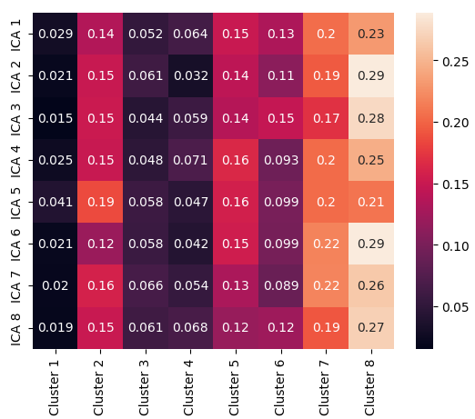
Figure 8: All of our independent components have a strong association with cluster 8.
Exporting to ONNX Format
The Open Neural Network Exchange (ONNX) protocol is an open-source and widely adopted industry protocol for building machine learning models that do not carry over any dependencies to the training framework or programming language that was used to implement the model. We will start by first importing the ONNX library.
import onnx
from skl2onnx.common.data_types import FloatTensorType
from skl2onnx import convert_sklearn
Then we will define the input and output shapes defined by our 3 ONNX models. These shapes are easy to retrieve; we simply call for the shapes of the matrices used to train these models. The final output of the last model is simply 1.
ica_embeddings_initial_types = [('float_input',FloatTensorType([1,train.loc[:,MA].shape[1]]))]
ica_embeddings_final_types = [('float_output',FloatTensorType([1,train.loc[:,MANIFOLD].shape[1]]))]

ica_forecast_initial_types = [('float_input',FloatTensorType([1,train.loc[:,MANIFOLD].shape[1]]))]
ica_forecast_final_types = [('float_output',FloatTensorType([1,train.loc[:,MANIFOLD].shape[1]]))]

returns_reconstruction_initial_types = [('float_input',FloatTensorType([1,train.loc[:,MANIFOLD].shape[1]]))]
returns_reconstruction_final_types = [('float_output',FloatTensorType([1,1]))]
We can finally save all 3 of our ONNX models to disk and import them into our MQL5 application.
onnx_proto = convert_sklearn(ica_embeddings_model,initial_types=ica_embeddings_initial_types,final_types=ica_embeddings_final_types,target_opset=12)
onnx.save(onnx_proto,'EURUSD ICA KNR.onnx')

onnx_proto = convert_sklearn(ica_forecast_model,initial_types=ica_forecast_initial_types,final_types=ica_forecast_final_types,target_opset=12)
onnx.save(onnx_proto,'EURUSD ICA F KNR.onnx')

onnx_proto = convert_sklearn(returns_reconstruction_model,initial_types=returns_reconstruction_initial_types,final_types=returns_reconstruction_final_types,target_opset=12)
onnx.save(onnx_proto,'EURUSD RR KNR.onnx')
Implementing Our Application in MQL5
To start implementing our application in MQL5, we will first load the ONNX files we need as resources for our application. The first 3 ONNX files we load have been built in this discussion, while the last ONNX file has been carried over from our previous discussion. It is the model that is responsible for determining which spectral cluster we are currently in.
//+------------------------------------------------------------------+
//|                                              ICA Filtering 3.mq5 |
//|                                  Copyright 2026, MetaQuotes Ltd. |
//|                                             https://www.mql5.com |
//+------------------------------------------------------------------+
#property copyright "Copyright 2026, MetaQuotes Ltd."
#property link      "https://www.mql5.com"
#property version   "1.00"

//+------------------------------------------------------------------+
//| Resources                                                        |
//+------------------------------------------------------------------+
#resource "\\Files\\ICA Filtering\\EURUSD ICA KNR.onnx" as const uchar onnx_ica_proto[];
#resource "\\Files\\ICA Filtering\\EURUSD ICA F KNR.onnx" as const uchar onnx_ica_forecast_proto[];
#resource "\\Files\\ICA Filtering\\EURUSD RR KNR.onnx" as const uchar onnx_returns_proto[];
#resource "\\Files\\ICA Filtering\\EURUSD SC KNR.onnx" as const uchar onnx_cluster_proto[];
Next, we will define the input and output variables for each ONNX model.
//+------------------------------------------------------------------+
//| Global variables                                                 |
//+------------------------------------------------------------------+
//--- Application variables
long        onnx_ica_model,onnx_returns_model,onnx_cluster_model,onnx_ica_forecast_model;
vectorf     onnx_ica_inputs,onnx_ica_outputs,onnx_ica_forecast_outputs,onnx_return_outputs,onnx_cluster_outputs;
The input and output shapes of each model are best defined once in the beginning of the application as constants. This ensures that consistent references will be made throughout our application and that we will not receive ONNX errors concerning the input and output shapes of our models.
//--- Fixed application variables
const int         ica_inputs = 24;
const int         ica_outputs = 8;
const int         returns_outputs = 1;
const int         cluster_outputs = 8;
const int         cluster_inputs = 24;
During our Python analysis, we calculated the average return associated with each dominant ICA component. These statistics will be helpful for our trading strategy, so we have loaded them in a globally scoped array.
//--- Statistical market variables
double component_returns[] = {-0.00036027072758037224,0.0007851651982378843,-0.0026335897435897444,0.0013590112994350295,
                              -0.0012734302325581438,0.0003883990719257571,0.00020506153846154207,0.0005790641247833572
                              };
On each new quote, we run four ONNX models sequentially: ICA manifold, ICA growth forecast, return reconstruction, and finally spectral cluster classification.
//+------------------------------------------------------------------+
//| Expert tick function                                             |
//+------------------------------------------------------------------+
void OnTick()
  {
//--- Update our time reading
   time_stamp = iTime(Symbol(),PERIOD_D1,1);
   static datetime previous_time_stamp;

   if(previous_time_stamp != time_stamp)
     {
      //--- Update the time stamp
      previous_time_stamp = time_stamp;

      //--- Fetch updated indicator readings
      if(!UpdateMarketData())
        {
         Print("An error occurred while trying to update indicator readings: ",GetLastError());
         return;
        }

      //--- Prepare the inputs for our ONNX models
      if(!FetchModelData())
        {
         Print("An error occurred while trying to fetch our ONNX model data: ");
         return;
        }

      //--- Approximate our ICA manifold
      if(!OnnxRun(onnx_ica_model,ONNX_DATA_TYPE_FLOAT,onnx_ica_inputs,onnx_ica_outputs))
        {
         Print("Failed to approximate ICA embedings: ",GetLastError());
         return;
        }

      //--- Forecast future ICA manifold growth
      else
         if(!OnnxRun(onnx_ica_forecast_model,ONNX_DATA_TYPE_FLOAT,onnx_ica_outputs,onnx_ica_forecast_outputs))
           {
            Print("Failed to forecast ICA embedings: ",GetLastError());
            return;
           }

         //--- Identify the cluster we are in
         else
            if(!OnnxRun(onnx_cluster_model,ONNX_DATA_TYPE_FLOAT,onnx_ica_inputs,onnx_cluster_outputs))
              {
               Print("Failed to identify Spectral Cluster: ",GetLastError());
               return;
              }

            else
              {
               //--- Forecast smoothed market returns from approximate ICA manifold
               if(!OnnxRun(onnx_returns_model,ONNX_DATA_TYPE_FLOAT,onnx_ica_forecast_outputs,onnx_return_outputs))
                 {
                  Print("Failed to forecast market returns: ",GetLastError());
                  return;
                 }

               else
                 {
                  SetupPosition();
                 }
              }
     }
  }
//+------------------------------------------------------------------+
The SetupPosition function is responsible for coordinating our position entries. This method will first check if we already have open positions in the market. When no open positions exist, the function calls the EnterTrade method. The EnterTrade method contains our trading logic and entry rules. Otherwise, if open positions do exist and the position's magic number matches the user's inputs, then the SetupPosition method will not call the EnterTrade method until our current position has reached maturity. The method is also responsible for resetting our trade_state flag to true if we have no open positions in the market.
//+------------------------------------------------------------------+
//| Check if we can enter a position                                 |
//+------------------------------------------------------------------+
void SetupPosition(void)
  {
   if(PositionSelect(Symbol()))
     {
      if(PositionGetInteger(POSITION_MAGIC) != magic_number)
        {
         Print("Attempting to execute trade.");
         trade_state = true;
         EnterTrade();
        }
     }

   else
      if(!PositionSelect(Symbol()))
        {
         Print("Attempting to execute trade.");
         trade_state = true;
         EnterTrade();
        }
  }
The logic our application follows for deciding which trade to enter has also changed considerably. We start by first identifying the current cluster we are in, and then we fetch the statistical properties associated with that cluster. Then we identify which ICA component is expected to grow the most and fetch returns we expect from that dominant component.
Recall that our ICA forecast model predicts the future growth expected in the ICA manifold. By taking the absolute values of this model's predictions, we can reproduce our Python analysis of determining which ICA component has grown the most. This is achieved by taking the absolute value of the model's output vector, followed by the ArgMax of the absolute value of the model's output vector. This renders the same results we relied on in our Python analysis.
If the expected cluster returns do not align with the expected return from the dominant component, then our strategy understands this discrepancy to be an indication of market noise. In this case, we will set a flag to false to stop our application from trading. Otherwise, if our application is granted permission to trade, then we will base our trading decisions based on the returns we expect to be associated with the growth in our ICA components.
//+------------------------------------------------------------------+
//| Execute our trade order                                          |
//+------------------------------------------------------------------+
void EnterTrade(void)
  {
//--- Let's keep track of the cluster expectations
   int current_cluster    = (int) onnx_cluster_outputs.ArgMax();
   double expected_cluster_return = cluster_returns[current_cluster];
   double expected_cluster_risk   = cluster_risk[current_cluster];
   onnx_ica_forecast_outputs = MathAbs(onnx_ica_forecast_outputs);
   int dominant_component = (int) onnx_ica_forecast_outputs.ArgMax();
   Print("Attempting to identify dominant component: ",dominant_component);
   double expected_component_return = component_returns[dominant_component];


//--- Check if market conditions are suitable for trading
   if(expected_cluster_return < 0 && expected_component_return > 0)
      trade_state = false;

   if(expected_cluster_return > 0 && expected_component_return < 0)
      trade_state = false;

//--- Long entries
   if((onnx_return_outputs[0] > 0) && trade_state)
     {
      //--- Best entry conditions possible
      if((expected_cluster_return > 0) && (expected_cluster_risk < average_cluster_risk))
        {
         Buy(0.03,2);
         return;
        }

      //--- Risky entry conditions, reduce the lot size and stop loss width
      else
         if((expected_cluster_return > 0) && (expected_cluster_risk > average_cluster_risk))
           {
            Buy(0.02,1.5);
            return;
           }

         //--- Worst possible entry conditions, use the smallest lot size and stop loss width
         else
           {
            Buy(0.01,1);
            return;
           }

     }

//--- Short entries
   else
      if((onnx_return_outputs[0] < 0) && trade_state)
        {
         //--- Best entry conditions possible
         if((expected_cluster_return < 0) && (expected_cluster_risk < average_cluster_risk))
           {
            Sell(0.03,2);
            return;
           }
         //--- Risky entry conditions, reduce the lot size and stop loss width
         else
            if((expected_cluster_return < 0) && (expected_cluster_risk > average_cluster_risk))
              {
               Sell(0.02,1.5);
               return;
              }
            //--- Worst possible entry conditions, use the smallest lot size and stop loss width
            else
              {
               Sell(0.01,1);
               return;
              }

        }
  }
The function that loads our ONNX models also requires revision. The changes made to it are small. We only need to add another model to the procedure. Then we will initialize the model from its ONNX buffer and ensure the model is valid. After validating the model, we will then define its input and output shapes and check these shapes have been defined correctly. Finally, we will then initialize zero vectors to store the future outputs of our models.
//+------------------------------------------------------------------+
//| Prepare our ONNX models for inferencing                          |
//+------------------------------------------------------------------+
bool LoadOnnxModels(void)
  {
//--- ONNX Models
   onnx_ica_model     = OnnxCreateFromBuffer(onnx_ica_proto,ONNX_DATA_TYPE_FLOAT);
   onnx_returns_model = OnnxCreateFromBuffer(onnx_returns_proto,ONNX_DATA_TYPE_FLOAT);
   onnx_cluster_model = OnnxCreateFromBuffer(onnx_cluster_proto,ONNX_DATA_TYPE_FLOAT);
   onnx_ica_forecast_model = OnnxCreateFromBuffer(onnx_ica_forecast_proto,ONNX_DATA_TYPE_FLOAT);

//--- Validate the ONNX model handlers
   if(onnx_ica_forecast_model == INVALID_HANDLE)
     {
      return(false);
     }

   if(onnx_cluster_model == INVALID_HANDLE)
     {
      return(false);
     }

   if(onnx_returns_model == INVALID_HANDLE)
     {
      return(false);
     }

   if(onnx_ica_model == INVALID_HANDLE)
     {
      return(false);
     }

//--- Validate the ONNX model shapes
   ulong onnx_ica_input_shape[] = {1,ica_inputs};
   ulong onnx_ica_output_shape[] = {1,ica_outputs};
   ulong onnx_returns_output_shape[] = {1,returns_outputs};
   ulong onnx_cluster_input_shape[] = {1,cluster_inputs};
   ulong onnx_cluster_output_shape[] = {1,cluster_outputs};

   if(!OnnxSetInputShape(onnx_ica_forecast_model,0,onnx_ica_output_shape))
     {
      Print("Failed to set the correct input shape for our ONNX forecast model.");
      return(false);
     }

   if(!OnnxSetOutputShape(onnx_ica_forecast_model,0,onnx_ica_output_shape))
     {
      Print("Failed to set the correct output shape for our ONNX forecast model.");
      return(false);
     }

   if(!OnnxSetInputShape(onnx_cluster_model,0,onnx_cluster_input_shape))
     {
      Print("Failed to set the correct ONNX Spectral Clustering model input shape: ",GetLastError());
      return(false);
     }


   if(!OnnxSetOutputShape(onnx_cluster_model,0,onnx_cluster_output_shape))
     {
      Print("Failed to set the correct ONNX Spectral Clustering model output shape: ",GetLastError());
      return(false);
     }

   if(!OnnxSetInputShape(onnx_ica_model,0,onnx_ica_input_shape))
     {
      Print("Failed to set the correct ONNX ICA model input shape: ",GetLastError());
      return(false);
     }


   if(!OnnxSetOutputShape(onnx_ica_model,0,onnx_ica_output_shape))
     {
      Print("Failed to set the correct ONNX ICA model output shape: ",GetLastError());
      return(false);
     }


   if(!OnnxSetInputShape(onnx_returns_model,0,onnx_ica_output_shape))
     {
      Print("Failed to set the correct ONNX smoothed returns model input shape: ",GetLastError());
      return(false);
     }

   if(!OnnxSetOutputShape(onnx_returns_model,0,onnx_returns_output_shape))
     {
      Print("Failed to set the correct ONNX smoothed returns model output shape: ",GetLastError());
      return(false);
     }

//--- Prepare ONNX model I/O
   onnx_ica_inputs = vectorf::Zeros(ica_inputs);
   onnx_ica_outputs = vectorf::Zeros(ica_outputs);
   onnx_return_outputs = vectorf::Zeros(returns_outputs);
   onnx_cluster_outputs = vectorf::Zeros(cluster_outputs);
   onnx_ica_forecast_outputs = vectorf::Zeros(ica_outputs);

//--- Everything went well
   return(true);
  }
When our application is no longer in use, we will release the resources that were previously committed to our application. This function is again altered only slightly, with the addition of one more call to release the model responsible for forecasting the growth in our ICA components.
//+------------------------------------------------------------------+
//| Free up all resources we are no longer using                     |
//+------------------------------------------------------------------+
bool ReleaseResources(void)
  {

   if(!OnnxRelease(onnx_ica_forecast_model))
     {
      Print("An error occurred when releasing the ONNX ICA Forecast model: ",GetLastError());
      return(false);
     }

   if(!OnnxRelease(onnx_cluster_model))
     {
      Print("An error occurred when releasing the ONNX Cluster model: ",GetLastError());
      return(false);
     }

   if(!OnnxRelease(onnx_ica_model))
     {
      Print("An error occurred when releasing the ONNX ICA model: ",GetLastError());
      return(false);
     }

   if(!OnnxRelease(onnx_returns_model))
     {
      Print("An error occurred when releasing the ONNX Smoothed Returns model: ",GetLastError());
      return(false);
     }

   return(true);
  }
//+------------------------------------------------------------------+
Testing Our Strategy in MQL5
We are now ready to start testing our trading strategy on out-of-sample historical market data. Let us first select test days that we will use to evaluate our trading strategy. Recall that these days were not shown to our statistical model during training. 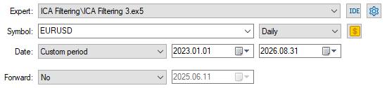
Figure 9: The back test days we will use to evaluate our trading strategy.
Now let us define the trading conditions that we will evaluate our model under. We want the most realistic emulation possible of market conditions; that's why we have set our delay settings to random delay, and our modeling of historical trading days will be based on real tick data retrieved from our broker. These settings may take a while to load depending on your network connectivity.
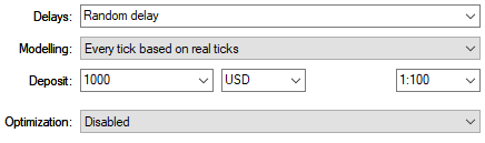
Figure 10: The test conditions we will employ aim to emulate real market conditions.
The equity curve produced by our trading strategy shows a positive trend in the account equity and balance over time. This gives us a measure of confidence that our indirect approach of modeling the market is a viable approach. Although our strategy cannot be considered the holy grail, it demonstrates that although our proposed piecewise solution is rather tedious to implement, it may be potentially well worth the effort exerted.
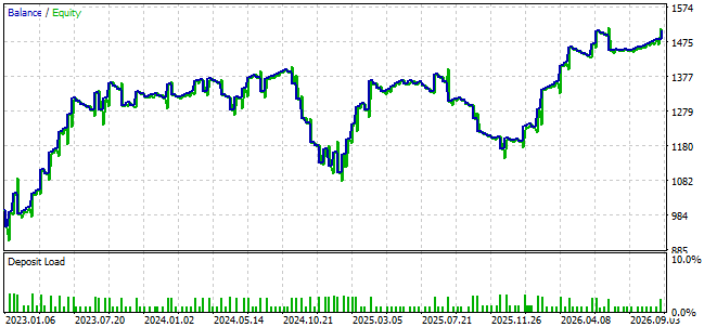
Figure 11: The equity curve produced by our piecewise forecasting strategy shows great promise.
We can also analyze a detailed statistical breakdown of our trading performance. Our Sharpe ratio on out-of-sample data was 0.81; this is encouraging to see because given the complexity of our strategy, we could've easily expected a low Sharpe ratio due to our model's falling out of step. Additionally, we can see that the econometric stats associated with our winning and losing positions are still strongly skewed in favor of our winning trades. Our largest and average profits were both considerably larger than their counterparts. Although our refined filter did not perfectly filter out all possible noise, it is a step in the right direction.
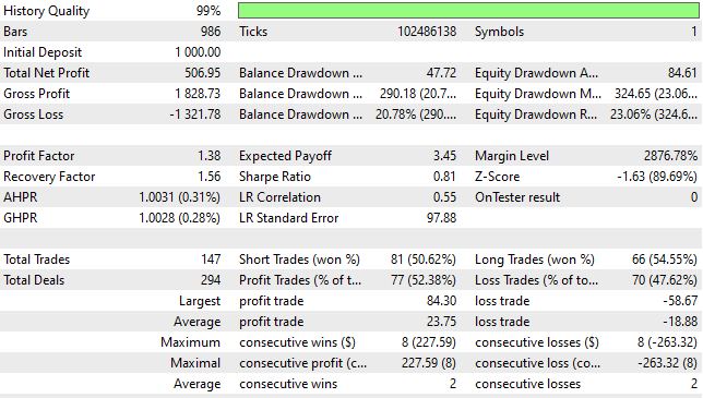
Figure 12: A detailed statistical table summarizes the performance of our suggested trading strategy.
Conclusion
We have now arrived at the end of our discussion. This article has furnished the reader with a reproducible statistical framework for filtering market noise embedded into historical market data. All the attached statistical ONNX models can be locally reproduced by the reader to render unique solutions that can be tailored to the reader's particular market and broker of interest. Our discussion here has furnished the reader with a powerful statistical pipeline for increasing signal-to-noise ratios.
Regularization is an important set of techniques used in machine learning to prevent overfitting. The topic is usually considered advanced and viewed generally as the domain of experts. The solution we have presented in our discussion uses the ICA algorithm as its own source of supervisory signals. This suggests to us that the target we are modeling is a function of the data we have. This is a part of the principles behind causality regularization. Implementing this solution is more involved but well worth the effort.
It is also worth mentioning that our new solution has its own unique set of potential weaknesses. One key possible failure point lies in the assumptions our strategy relies on. We assumed that the average effect associated with the growth in each independent component is stationary; this may not always be the case. Additionally, our strategy currently has 3 ONNX models that share their outputs. This may allow for compounding errors if market conditions are particularly volatile. If the reader has sufficient data, a longer backtest period may be advisable.
| File Name | File Description |
|---|---|
| ICA Filtering 3.mq5 | The expert advisor we built together that uses the forecasted growth in the ICA components as the basis of its forecast. |
| EURUSD_ICA_KNR.onnx | The ONNX model responsible for approximating ICA embeddings from current market readings. |
| EURUSD_ICA_F_KNR.onnx | This is the ONNX model we employed to forecast the growth in each ICA component. |
| EURUSD_RR_KNR.onnx | The ONNX model that we relied on to reconstruct the smoothed market returns from forecasted ICA component growth. |
| EURUSD_SC_KNR.onnx | This ONNX model helped us determine which spectral cluster we are currently in. |
| ICA_Forecasting.ipynb | The Jupyter Notebook we used to analyze our historical market data. |
| ICA Filtering.mq5 | The MQL5 script we implemented to fetch historical market data. |
Warning: All rights to these materials are reserved by MetaQuotes Ltd. Copying or reprinting of these materials in whole or in part is prohibited.
This article was written by a user of the site and reflects their personal views. MetaQuotes Ltd is not responsible for the accuracy of the information presented, nor for any consequences resulting from the use of the solutions, strategies or recommendations described.

 RSI Divergence Grid Expert Advisor with Risk Manager in MQL5
 Markowitz Mean-Variance Optimization for MQL5: A Native Efficient-Frontier Portfolio Builder
 Features of Experts Advisors
 Neural Networks in Trading: Recurrent Modeling of Market Micromovements (Encoder)

- Free trading apps
- Over 8,000 signals for copying
- Economic news for exploring financial markets
You agree to website policy and terms of use