Kohonen Self-Organizing Maps in an MQL5 Expert Advisor

Introduction: In Search of an Invisible Order

Imagine you are looking at a chart for a currency pair. Thousands of candles, millions of data points, an endless stream of numbers. Somewhere within this chaos lie patterns, regularities, and recurring structures. But the human brain cannot keep thousands of candles in mind at the same time and find connections between them. We need a map of this chaos. We need a framework that will show where similar market situations cluster together and where something fundamentally new begins.

This is exactly why Finnish scientist Teuvo Kohonen invented self-organizing maps — Self-Organizing Maps, or SOM — in 1982. This is not just another neural network. This is a way to make a computer see an invisible data structure, find order in chaos, and create a two-dimensional map of a multidimensional space. And what is most interesting is that this technology, developed forty years ago for speech recognition, turned out to be ideally suited for analyzing financial markets.

What Are Self-Organizing Maps: The Geography of Market Chaos

Let's start with a simple analogy. Imagine that you are a geographer and you are tasked with creating a map of an unknown area. You have the coordinates of thousands of points, as well as measurements of elevation, temperature, and humidity — a wide range of parameters for each point. How can we turn this jumble of numbers into an easy-to-understand two-dimensional map, where similar places are close together and different ones are far apart?

The Kohonen self-organizing map does exactly that, but with market data. We have a multidimensional space of features — prices, volumes, volatility, changes over various periods, and technical indicators. Each candlestick on the chart represents a point in this multidimensional space. A SOM maps all these points and projects them onto a two-dimensional grid of neurons, while preserving the topology — similar market situations end up in neighboring neurons on the map.

The magic begins during the training process. The network consists of a two-dimensional grid of neurons, for example, twenty by twenty — four hundred neurons. Each neuron has a weight vector with the same dimensionality as the input data. When we present the network with a new pattern from the market, it finds the neuron with the most similar weights — this is called the Best Matching Unit, or BMU. Then the magic happens: not only does the BMU update its weights to become even more similar to the input pattern, but its neighbors on the map also shift in the same direction. The farther away from the BMU, the weaker the influence.

After being trained on thousands of market situations, the map self-organizes. Neurons in one corner of the map may be responsible for strong bullish trends, in another corner for bearish declines, and in the middle for sideways markets and uncertainty. The map creates a kind of geography of market states, where the distance between neurons reflects the degree of difference between patterns.

Why SOMs Are Ideal for Trading: The Advantages of Topology

Traditional neural networks for classification, such as multilayer perceptrons or convolutional networks, are essentially black-box models. You feed them data, they produce a prediction, but what happens inside is a mystery. SOMs are different. They provide you with visualization, understanding, and structure. You can look at the map to see where the current market situation falls within the pattern space. You can track how the market moves across the map from one state to another.

Even more importantly, SOMs preserve topology. If two market patterns are similar, they will end up in adjacent neurons. This means that the network does not just classify — it clusters, groups, and identifies natural boundaries between different types of market behavior. This is unsupervised learning. You do not need to label the data in advance into classes such as "bullish trend," "bearish trend," and "sideways market." The network will identify these classes on its own and determine the boundaries between them.

SOMs are also robust to noise. Market data is noisy by definition — random outliers, gaps, manipulation, and news-driven surges. Conventional neural networks can overfit to this noise. SOMs, thanks to updates across neuron neighborhoods, average out noise and identify robust patterns.

SOM Architecture in MQL5: Creating a Neural Map

Let's take a look at how the self-organizing map is implemented in the Expert Advisor code. We will start with the basic parameters:

#define SOM_WIDTH 20
#define SOM_HEIGHT 20
#define SOM_NEURONS (SOM_WIDTH * SOM_HEIGHT)

struct QuantumProcessor {
    matrix som_weights;           // SOM weights [SOM_NEURONS x input_dim]
    double learning_rate_som;
    double neighborhood_radius;
    
    void Init() {
        learning_rate_som = 0.1;
        neighborhood_radius = 5.0;
        som_weights = matrix::Zeros(SOM_NEURONS, FEATURES_COUNT);
        InitializeRandomMatrix(som_weights, -0.5, 0.5);
    }

A twenty-by-twenty-neuron map gives us four hundred points in the classification space. Each neuron has a weight vector of dimension FEATURES_COUNT — 400 features extracted from market data. Initializing the weights with random values ranging from minus one-half to plus one-half creates initial diversity in the map.

Key training parameters: learning rate 0.1 and neighborhood radius 5.0. The neighborhood radius determines how far from the Best Matching Unit the influence extends when the weights are updated. A large radius at the beginning of training allows the map to organize itself at a coarse level. As training progresses, the radius can be gradually reduced for fine-tuning.

Finding the Best Matching Unit: The Heart of the Algorithm

The most important operation in an SOM is finding the neuron that most closely resembles the input pattern:

int FindBestMatchingUnit(const vector &_input) {
    int bmu = 0;
    double min_distance = DBL_MAX;
    
    for(int i = 0; i < SOM_NEURONS; i++) {
        vector neuron_weights = som_weights.Row(i);
        double distance = 0.0;
        
        for(ulong j = 0; j < MathMin(_input.Size(), neuron_weights.Size()); j++) {
            double diff = _input[j] - neuron_weights[j];
            distance += diff * diff;
        }
        
        if(distance < min_distance) {
            min_distance = distance;
            bmu = i;
        }
    }
    return bmu;
}

The algorithm is simple and elegant. We iterate through all 400 neurons in the map, and for each one, we calculate the Euclidean distance between the neuron's weights and the input vector. The squared distance is computed faster than taking the square root, and that is sufficient for comparison purposes. The neuron with the shortest distance becomes the winner — the BMU.

This is an operation with linear complexity in the number of neurons. For a 20-by-20 map with 400 features, a single BMU search iteration requires 160,000 multiplication and addition operations. On modern processors, this is done in microseconds. It is important to note that this operation is deterministic — for the same input, the same BMU will always be found (provided the weights have not changed).

Weight Update: The Dance of Neurons

Once the BMU has been found, the most interesting part begins — updating the neighborhood weights:

void UpdateSOMWeights(const vector &_input, int bmu) {
    int bmu_x = bmu % SOM_WIDTH;
    int bmu_y = bmu / SOM_WIDTH;
    
    for(int i = 0; i < SOM_NEURONS; i++) {
        int neuron_x = i % SOM_WIDTH;
        int neuron_y = i / SOM_WIDTH;
        
        double distance = MathSqrt((neuron_x - bmu_x) * (neuron_x - bmu_x) + 
                                 (neuron_y - bmu_y) * (neuron_y - bmu_y));
        
        if(distance <= neighborhood_radius) {
            double influence = MathExp(-(distance * distance) / 
                              (2.0 * neighborhood_radius * neighborhood_radius));
            
            for(ulong j = 0; j < MathMin(_input.Size(), som_weights.Cols()); j++) {
                som_weights[i][j] += learning_rate_som * influence * 
                                   (_input[j] - som_weights[i][j]);
            }
        }
    }
}

The code implements the classic Gaussian kernel neighborhood function. First, we calculate the coordinates of the BMU on a two-dimensional map — the index modulo the width gives the x-coordinate, and integer division by the width gives the y-coordinate. Next, for each neuron, we compute the Euclidean distance to the BMU in the map coordinates (not in feature space!).

If the distance is less than the neighborhood radius, the neuron falls within the area of influence. The degree of influence is determined by a Gaussian function — an exponential of the negative square of the distance. At the center (the BMU itself), the influence is maximal and equal to one. At the edge of the radius, the influence drops almost to zero. This smooth function creates a smooth topology — neurons are updated in proportion to their proximity to the winner.

The final learning rule is the classic delta rule. The new weight equals the old weight plus the learning rate multiplied by the influence and by the difference between the input and the current weight. This rule pulls the neuron's weight vector toward the input vector. The closer a neuron is to the BMU, the stronger the attraction. The farther away it is, the weaker the attraction.

Integrating SOM into a Trading System: Quantum Effects

A key feature of the implementation in the Expert Advisor is the integration of SOM as part of a "quantum processor," which adds extra effects on top of the base SOM:

matrix ApplyQuantumEffects(const matrix &input_data, const matrix &context_data) {
    matrix result = matrix::Zeros(input_data.Rows(), input_data.Cols());
    
    for(ulong i = 0; i < input_data.Rows(); i++) {
        vector input_row = input_data.Row(i);
        
        // Find the BMU for the current input
        int bmu = FindBestMatchingUnit(input_row);
        
        // Update the SOM weights
        UpdateSOMWeights(input_row, bmu);
        
        // Get the activation from the BMU
        vector bmu_weights = som_weights.Row(bmu);
        
        // Apply classical effects + SOM activation
        for(ulong j = 0; j < input_data.Cols(); j++) {
            double input_val = input_data[i][j];
            double context_val = (i < context_data.Rows() && j < context_data.Cols()) ? 
                                context_data[i][j] : 0.0;
            
            // SOM effect
            double som_factor = 1.0;
            if(j < bmu_weights.Size()) {
                som_factor += (bmu_weights[j] - input_val) * coherence * 0.1;
            }
            
            // Classical effects
            double resonance = 1.0 + resonance_strength * 
                             MathCos(input_val * context_val * M_PI);
            double interference = interference_amplitude * 
                                MathSin(input_val * context_val * 2.0 * M_PI);
            double coherent_factor = coherence + (1.0 - coherence) * 
                                   MathExp(-decoherence_rate * i);
            
            result[i][j] = input_val * resonance * coherent_factor * 
                         som_factor + interference;
        }
    }
    
    return result;
}

The term "quantum effects" is, of course, a metaphor. There is no real quantum computing going on here. But it is an interesting idea: additional transformations are applied to the SOM output to simulate resonance, interference, and coherence. SOM identifies similar patterns and groups them, while additional effects introduce nonlinearity and contextual dependence.

The SOM effect calculates the difference between the BMU weights and the input data, multiplies it by the coherence parameter, and adds it to the base coefficient. This creates a feedback loop: if the current pattern is far from the cluster center (the BMU weights), the output is amplified or weakened. Resonance is modeled using the cosine of the product of the input and the context. Interference is added as a sinusoidal component. The coherence factor decays exponentially with the index, simulating memory loss.

Training on Historical Data: From Bars to Patterns

The Expert Advisor training process begins when the EA is initialized:

void TrainSOMNetwork() {
    matrix training_data = matrix::Zeros(TrainingBars, FEATURES_COUNT);
    vector targets = vector::Zeros(TrainingBars);
    
    MqlRates rates[];
    ArraySetAsSeries(rates, true);
    
    if(CopyRates(Symbol(), Period(), 0, TrainingBars + 50, rates) < TrainingBars + 50) {
        Print("Failed to copy rates for training");
        return;
    }
    
    for(int i = 0; i < TrainingBars; i++) {
        vector features = vector::Zeros(FEATURES_COUNT);
        
        // Basic Features
        double price_change = (rates[i].close - rates[i].open) / rates[i].open;
        double volatility = 0.0;
        for(int j = i; j < i + 10 && j < ArraySize(rates); j++) {
            double change = (rates[j].close - rates[j].open) / rates[j].open;
            volatility += change * change;
        }
        volatility = MathSqrt(volatility / 10.0);
        
        double volume_ratio = (rates[i].tick_volume > 0) ? 
            MathLog(1.0 + rates[i].tick_volume / 1000.0) : 0.0;
        
        features[0] = MathMax(-1.0, MathMin(1.0, price_change * 100));
        features[1] = MathMax(0.0, MathMin(1.0, volatility * 100));
        features[2] = MathMax(0.0, MathMin(1.0, volume_ratio / 10.0));

The first three features are basic. The current bar's price change, normalized to the range from minus one to plus one. Volatility over the last ten bars, calculated as the standard deviation of price changes and normalized to the range from zero to one. Volume on a logarithmic scale, also normalized.

Additional features are then added — price changes and ranges for the previous twenty bars — creating a time window for analyzing short-term history. In total, there are four hundred features per bar. This is a multidimensional representation of market conditions that the SOM will learn to cluster.

Creating Targets: Predicting the Future

The key step in training is defining the target variable. What do we want to predict?

// NEW TARGET: price change after N bars (default: 24)
if(i + TargetBarsLookahead < ArraySize(rates)) {
    double current_price = rates[i].close;
    double future_price = rates[i + TargetBarsLookahead].close;
    double price_change_percent = (current_price - future_price) / future_price * 100.0;
    
    // Define the target based on configurable thresholds
    if(price_change_percent > BullishThreshold) {        // Rise Exceeds the Threshold
        targets[i] = 0.8;
    }
    else if(price_change_percent < BearishThreshold) {   // Decline Exceeds the Threshold
        targets[i] = 0.2;
    }
    else {                                               // Sideways Market
        targets[i] = 0.5;
    }
}

The system looks ahead by a customizable number of bars (the default is twenty-four) and calculates the percentage change in price. If the change exceeds the rise threshold (0.5 percent by default), the target is set to 0.8 — a strong bullish signal. If the price change is below the threshold (-0.5 percent by default), the target is 0.2 — a strong bearish signal. Everything else is classified as a sideways market with a target of 0.5.

This three-class classification gives the network clear training targets. The SOM groups market situations that lead to a rise in one area of the map, situations preceding a decline in another area, and uncertainty in a third. After being trained on thousands of examples, the map becomes a predictive tool.

The Prediction Process: From Features to a Signal

When the Expert Advisor receives a new tick, it extracts the features and makes a prediction:

double GetSOMPrediction(double &confidence) {
    vector feature_data = vector::Zeros(FEATURES_COUNT);
    
    MqlRates rates[];
    ArraySetAsSeries(rates, true);
    
    if(CopyRates(Symbol(), Period(), 0, 50, rates) < 50) {
        Print("Failed to copy rates");
        return -1;
    }
    
    // Populate the features
    double price_change = (rates[0].close - rates[1].close) / rates[1].close;
    double volatility = 0.0;
    for(int i = 0; i < 10; i++) {
        double change = (rates[i].close - rates[i].open) / rates[i].open;
        volatility += change * change;
    }
    volatility = MathSqrt(volatility / 10.0);
    
    double volume_ratio = (rates[0].tick_volume > 0) ? 
        MathLog(1.0 + rates[0].tick_volume / 1000.0) : 0.0;
    
    feature_data[0] = MathMax(-1.0, MathMin(1.0, price_change * 100));
    feature_data[1] = MathMax(0.0, MathMin(1.0, volatility * 100));
    feature_data[2] = MathMax(0.0, MathMin(1.0, volume_ratio / 10.0));
    
    return g_som_net.Predict(feature_data, confidence);
}

Feature extraction is identical to what was done during training — price changes, volatility, volume, plus historical values. The feature vector is passed to the neural network's Predict method, which goes through the entire architecture: the SOM identifies the BMU, quantum effects are applied, the data is processed by transformer blocks, and the output is a prediction ranging from zero to one.

A value close to 0.8 means that the current market situation is similar to situations in the training set that were followed by a rise. A value close to 0.2 indicates a likely decline. A value around 0.5 indicates uncertainty — the market is moving sideways or is on the verge of a reversal.

Signal Processing and Opening Positions

The trading decision-making logic is based on the prediction and model confidence:

void ProcessSignals(double prediction, double confidence) {
    if(TimeCurrent() - g_last_signal_time < PeriodSeconds(Period())) return;
    
    int positions = CountPositions();
    
    if(confidence >= MinConfidence && prediction >= 0.6 && positions == 0) {
        if(OpenPosition(ORDER_TYPE_BUY)) {
            g_last_signal_time = TimeCurrent();
            Print("SOM BUY: Prediction=", DoubleToString(prediction*100,1), 
                  "%, Confidence=", DoubleToString(confidence*100,1), "%");
        }
    }
    else if(confidence >= MinConfidence && prediction <= 0.4 && positions == 0) {
        if(OpenPosition(ORDER_TYPE_SELL)) {
            g_last_signal_time = TimeCurrent();
            Print("SOM SELL: Prediction=", DoubleToString(prediction*100,1), 
                  "%, Confidence=", DoubleToString(confidence*100,1), "%");
        }
    }
}

The Expert Advisor opens a position only if three conditions are met: the model confidence is above the minimum threshold (65 percent by default), the prediction is strong enough (above 0.6 for a buy or below 0.4 for a sell), and there are no open positions. This cautious approach minimizes false entries.

The confidence parameter is calculated by a meta-model that assesses how reliable the current prediction is, based on the model's historical accuracy and the features of the current pattern. Low confidence may mean that the pattern does not resemble anything in the training set — the model is in uncharted territory, and it is best to refrain from trading.

Continuous Learning: Adapting to the Market

Markets change. Patterns that worked a year ago may become obsolete. That is why the advisor supports continuous learning:

input bool     ContinuousLearning = true; // Retrain periodically
input int      RetrainHours = 12;        // Retrain every N hours

void OnTick() {
    if(!g_net_initialized) return;
    if(!IsNewBar()) return;
    
    if(ContinuousLearning && ShouldRetrain()) {
        Print("Retraining SOM...");
        TrainSOMNetwork();
        g_last_retrain_time = TimeCurrent();
        Print("SOM retrained!");
    }

Every twelve hours (this setting is configurable), the Expert Advisor runs a retraining process using the latest historical data. The SOM map is updated, adapting to new market conditions. Old patterns are not completely forgotten — the weights of the neurons change gradually, preserving the accumulated structure while incorporating new information.

This mechanism is critical to the long-term stability of the trading system. A static model that has been trained only once will degrade sooner or later. An adaptive model that continuously learns from new data remains relevant.

Visualizing a SOM Map: Seeing the Invisible

One of the main advantages of a SOM is that it can be visualized. After training, you can construct a U-matrix (unified distance matrix), which shows the distances between neighboring neurons. The dark areas on the U-matrix represent the boundaries between clusters, while the light areas represent homogeneous regions with similar patterns.

You can also color the map based on the average target values mapped to each neuron. Red neurons represent bearish patterns, green neurons represent bullish patterns, and gray neurons represent a sideways market. This map becomes a tool for the trader: by seeing which neuron the current situation falls into, you can immediately assess the likely direction of price movement.

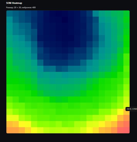
In the Expert Advisor implementation, visualization is handled by exporting an interactive HTML map — a SOM heat map with hover tooltips and zoom functionality. This is a standalone web page generated in MQL5 without any external libraries. After training (or when the 'H' hotkey is pressed on the chart), the ExportSOMHTML method calculates the L2 norm of each neuron's weight vector (as a measure of a cluster's "strength" or structural density), normalizes the values to [0..1], and saves an HTML file to the terminal’s common directory (Common\Files\SOM_map.html).

The export code is simple and effective:

bool ExportSOMHTML(const string filename = "SOM_map.html") {
    // Initialization Check
    if(input_quantum_proc.som_weights.Rows() != SOM_NEURONS) {
        Print("ExportSOMHTML: som_weights not initialized");
        return false;
    }
    
    // Calculation of L2 Norms for a Heat Map
    vector vals = vector::Zeros(SOM_NEURONS);
    double vmin = DBL_MAX, vmax = -DBL_MAX;
    for(int i = 0; i < SOM_NEURONS; i++) {
        double s = 0.0;
        for(ulong j = 0; j < input_quantum_proc.som_weights.Cols(); j++) {
            double w = input_quantum_proc.som_weights[i][j];
            s += w * w;
        }
        s = MathSqrt(s);
        vals[i] = s;
        if(s < vmin) vmin = s;
        if(s > vmax) vmax = s;
    }
    
    // Normalization and Saving the HTML
    double range = (vmax > vmin) ? (vmax - vmin) : 1.0;
    int h = FileOpen(filename, FILE_WRITE | FILE_TXT | FILE_COMMON, CP_UTF8);
    if(h == INVALID_HANDLE) {
        Print("ExportSOMHTML: cannot open file: ", filename);
        return false;
    }
    
    // Generating HTML with Canvas and JavaScript for Rendering
    // ... (complete HTML code with an HSL color palette ranging from blue to red, hover support, and resizing)
    
    FileClose(h);
    Print("SOM map exported to Common\\Files\\", filename);
    return true;
}

The file can be opened by double-clicking it in the MT5 terminal or in any browser. A 20×20-cell map is colored from “cool” blue (low weight norm — weak/empty clusters) to “hot” red (high weight norm — dense, active patterns). Hover your cursor over a cell to see its (x, y) coordinates and normalized intensity (0.0000–1.0000). Scaling is adaptive: cells are larger on a big screen and more compact on a mobile device.

This visualization is key to interpreting the model. For example, if the current BMU falls into a “hot” red zone with a high norm, this signals a strong cluster of patterns (bullish or bearish). If it is in the blue zone, the market is in a rare, uncertain zone where it is best not to trade.

Comparison with Other Methods: Where SOM Excels

Classic technical analysis uses predefined indicators — RSI, MACD, and Bollinger Bands. These indicators were developed by people based on hypotheses about market behavior. SOM makes no assumptions in advance. It learns from the data and identifies patterns that actually work, rather than the ones we merely think work.

Simple feedforward neural networks require labeled data — for each example, you must specify the correct answer. SOM is a form of unsupervised learning — learning without a teacher. It can also operate in supervised mode (as in our Expert Advisor), but its main strength lies in its ability to find structure in the data on its own.

Deep neural networks (LSTM, GRU, transformers) require enormous amounts of data and computational resources. SOM is compact and fast, and can be trained even on small datasets. Four hundred map neurons can be trained in a matter of minutes on a standard computer, and predictions are made in milliseconds.

Random Forest and gradient boosting work very well with tabular data, but they do not preserve topology very well. They create decision trees that divide the feature space into rectangular regions. SOM creates a smooth, continuous map in which similar patterns are located close to one another. This property is critically important for financial data, where small changes in features should not lead to abrupt jumps in predictions.

Limitations and Challenges: Reality Versus Theory

Like any technology, SOM is not a panacea. The first problem is the size of the map. A map that is too small (for example, ten by ten neurons) will not be able to capture the full complexity of market patterns. A map that is too large (say, one hundred by one hundred neurons) will overfit and be slow to train. The optimal size is determined experimentally.

The second issue is the number of training epochs. Too few epochs, and the map will not have time to organize itself; too many, and overfitting will occur. Our Expert Advisor uses only three epochs during continuous learning, which is a compromise between adaptation and stability.

The third problem is feature normalization. The SOM is sensitive to the scale of the data. If one feature has values ranging from zero to 100 and another from zero to one, the first feature will dominate when distances are calculated. All features must be carefully normalized to the same range.

The fourth problem is temporal dependence. A classical SOM does not take the temporal order of the data into account — each pattern is processed independently. For financial time series, this is a limitation. Our Expert Advisor partially solves this problem by adding historical lags to the features and integrating the SOM with transformer blocks that process sequences.

Future Directions: Where to Go From Here

Self-organizing maps are just the beginning. There are modifications of the classical Kohonen algorithm that can be integrated into the Expert Advisor. For example, Growing Neural Gas is an algorithm that dynamically adds and removes neurons during training, automatically adjusting the size of the map to match the complexity of the data.

Temporal Kohonen Maps add temporal connections between neurons, allowing the map to remember not only patterns but also sequences of patterns. This is critically important for predicting market trends, where it is not only the current situation that matters, but also the path the market took to reach it.

Hierarchical SOMs create multiple levels of maps, where the upper level groups lower-level neurons into meta-clusters. This makes it possible to capture market structure across different time scales — from minute-by-minute fluctuations to weekly trends.

Integrating SOMs with other deep learning techniques opens up even more possibilities. You can use a SOM as the first feature-extraction layer before an LSTM network. It is possible to train ensembles of SOMs on different timeframes and combine their predictions. Reinforcement learning can be applied on top of a SOM, where the agent learns trading strategies using market states classified by the map.

Practical Recommendations: How to Use the Expert Advisor

If you decide to test or use the SOM Expert Advisor, start by carefully configuring the training parameters. The TrainingBars parameter specifies how many historical bars to use for training: 2,000 is the minimum; 4,000 is better. TargetBarsLookahead defines the forecast horizon — twenty-four bars on an hourly chart means a forecast for one day ahead.

The BullishThreshold and BearishThreshold parameters are critical. Thresholds that are too low (for example, 0.1 percent) will result in a large number of weak signals. If the thresholds are set too high (for example, 2 percent), the signals will be infrequent. The optimal values depend on the instrument's volatility and the time frame.

The MinConfidence parameter filters out weak predictions. A value of 0.65 means that the Expert Advisor will trade only when model confidence is above 65 percent. This reduces the number of trades but improves their quality. When backtesting, look at the relationship between the win rate and the profit factor at different values of this parameter.

Be sure to use continuous learning (ContinuousLearning = true) when trading on a live account. Markets evolve, and a static model will quickly become outdated. The RetrainHours = 12 parameter means retraining twice a day, which strikes a reasonable balance between adaptation and stability.

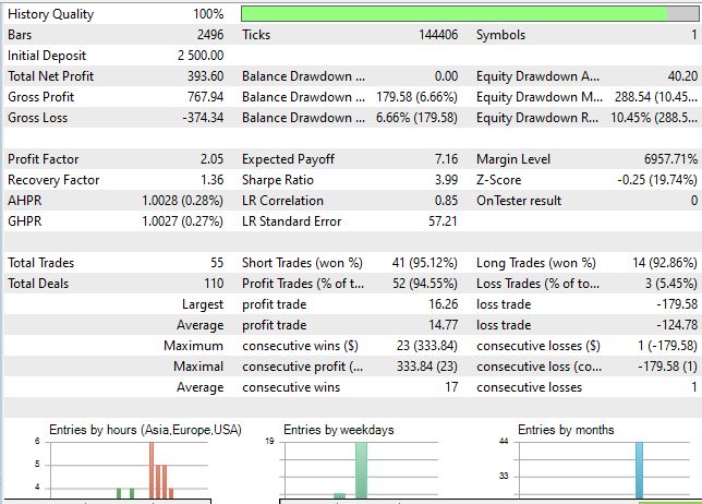
Now let's look at a test of our system:

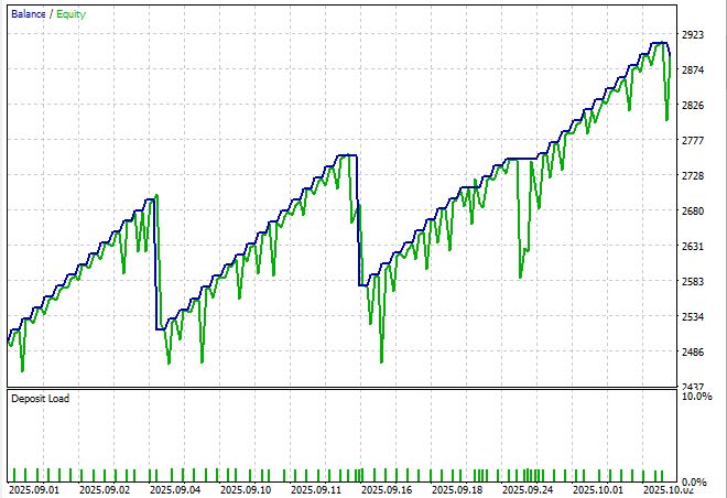
The equity curve is not particularly pretty, but then again, this is without any optimization, with the parameters set at random. And yet, the Sharpe ratio almost reached 4:

Conclusion: Neural Cartography of Finance

Kohonen's self-organizing maps are an elegant tool for analyzing complex, multidimensional data. Developed forty years ago for speech recognition, they have found applications in hundreds of fields — from bioinformatics to sociology. And as it turns out, they are very well suited to analyzing financial markets.

The Expert Advisor whose code we analyzed demonstrates one way to apply SOM in algorithmic trading. This is not a ready-made trading system, but a research platform that demonstrates the technology's capabilities. Live trading will require additional work — backtesting on historical data, parameter optimization, integration with a risk management system, and psychological readiness for drawdowns.

But the most important thing is the concept. The idea that the market can be mapped, that the chaos of candlesticks on the chart hides an orderly structure that can be identified and used. SOM provides us with a tool for creating this map. A map that shows where we are in the space of market states and where we are likely to move next.

The code is publicly available. The technology is available. All that is left is to apply it wisely, patiently, and with due caution. Markets do not forgive overconfidence, but they reward those who use the right tools the right way. Perhaps self-organizing maps will become your tool for navigating the ocean of financial data.