Creating a Probabilistic Market-Neutral Trading Robot Based on a Return Distribution

Most traders try to predict the market's direction, and most lose money. There is another approach: instead of trying to predict direction, use the statistical properties of the market itself. A market-neutral strategy based on the distribution of returns works exactly this way: it places orders at levels where the price is statistically likely to be, regardless of the trend.

Foundation: Return Distribution

Return is the percentage change in price over a fixed period. If the price was 1.0850 and rose to 1.0900, the return is equal to (1.0900 - 1.0850) / 1.0850 = 0.0046, or 0.46%. If you take all the historical returns from past periods and plot a histogram, you get a return distribution. For currency pairs, this distribution is typically close to a normal distribution, with the center of the distribution around zero and heavy tails.

For example, here is a histogram of the return distribution on the hourly EURUSD chart over 11 years, starting in January 2014:

Here is the cumulative distribution, and here we can already see the notorious “fat tails” of the distribution — as one of the reasons for the asymmetry between profit and risk, as well as one of the reasons why forecasting the market as a whole is so difficult: extreme movements occur much more frequently than a normal distribution would predict. If returns followed a classic bell-shaped Gaussian curve, the probability of a move of more than 1% in 10 hours would be negligible, but actual data show that such events occur regularly.

This is precisely why strategies based on the assumption of normality systematically underestimate the risk of catastrophic losses and overestimate the frequency of small profitable moves, making statistical arbitrage a more complex — but also a more honest — approach: we work with the actual empirical distribution, rather than its idealized mathematical model.

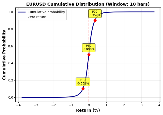
Key idea: if we know the return distribution covering 90% of observed returns over a given time window, we can predict not the direction, but the probability of reaching specific price levels. This is a fundamentally different trading philosophy.

Instead of asking, "Where will the price go?", we ask, "What is the probability that the price will reach a certain level within N periods?" The difference is crucial: the first question requires knowledge of the future, while the second relies on past statistics. If the empirical distribution shows that in 10% of cases the price falls by 0.5% or more within 10 hours, we can place a BUY LIMIT order at that level, knowing that the probability of it being triggered is about 10%. We do not know exactly when this will happen, but we do know that it will happen with a certain frequency.

This logic reverses the traditional approach to money management. A classic strategy uses large position sizes for “reliable” signals and small ones for “questionable” signals. The statistical approach does the opposite: small position sizes are used for high-probability central levels (they are triggered frequently but generate small profits), while large position sizes are used for low-probability tail levels (they are triggered rarely but generate large profits). The math balances frequency and magnitude through inverse probability weighting.

Moreover, by using a full distribution rather than point forecasts, the strategy naturally becomes market-neutral. We place orders across the entire range of possible price movements — both up and down — with order sizes proportional to their statistical rarity. This is not hedging in the traditional sense; rather, it is an acknowledgment of the fundamental uncertainty of direction while simultaneously leveraging the statistical certainty of the distribution.

Let's start by creating a structure to store the statistics:

struct ReturnStats {
   double mean;              // Average return
   double stdDev;            // Standard deviation
   double percentiles[10];   // P10, P20, ..., P100
};

ReturnStats returnStats;
double returns[];
bool statsCalculated = false;

The mean reflects the overall trend over the window (usually close to zero for short periods); the standard deviation indicates volatility; and the percentiles are quantiles of the distribution that divide it into equal parts by probability.

Calculation of the Empirical Distribution

The calculation function loads historical data and computes returns over a rolling window:

bool CalculateReturnDistribution() {
   MqlRates rates[];
   ArraySetAsSeries(rates, true);
   
   int copied = CopyRates(_Symbol, PERIOD_CURRENT, 0, HistoryBars + WindowBars, rates);
   if(copied < HistoryBars + WindowBars) {
      Print("ERROR: Not enough history. Got ", copied, " bars");
      return false;
   }
   
   int numReturns = HistoryBars;
   ArrayResize(returns, numReturns);
   
   for(int i = 0; i < numReturns; i++) {
      double priceStart = rates[i + WindowBars].close;
      double priceEnd = rates[i].close;
      
      if(priceStart > 0) {
         returns[i] = (priceEnd - priceStart) / priceStart;
      } else {
         returns[i] = 0;
      }
   }

For each point in the history, we take the closing price of the current bar and the closing price from WindowBars bars ago. The return is calculated as a relative change. If you set WindowBars = 10 on the M5 chart, you will get the return over 50 minutes. On the H1 chart, this represents the return over a 10-hour period.

After calculating all the returns, we sort the array to extract the percentiles:

double sortedReturns[];
   ArrayResize(sortedReturns, numReturns);
   ArrayCopy(sortedReturns, returns);
   ArraySort(sortedReturns);
   
   returnStats.mean = 0;
   for(int i = 0; i < numReturns; i++) {
      returnStats.mean += returns[i];
   }
   returnStats.mean /= numReturns;
   
   double variance = 0;
   for(int i = 0; i < numReturns; i++) {
      double diff = returns[i] - returnStats.mean;
      variance += diff * diff;
   }
   returnStats.stdDev = MathSqrt(variance / numReturns);
   
   for(int i = 0; i < 10; i++) {
      double percentileLevel = (i + 1) * 0.10;
      int index = (int)(numReturns * percentileLevel);
      if(index >= numReturns) index = numReturns - 1;
      returnStats.percentiles[i] = sortedReturns[index];
   }
   
   statsCalculated = true;
   return true;
}

Percentiles are extracted by simple indexing of the sorted array. P10 is the element at the index equal to 10% of the array length. P90 is the element at the 90% index. We obtain exact quantiles of the empirical distribution without making any assumptions about its shape. This is important: we do not assume normality; we use the data as it is.

The Mathematics of Weighting Factors

If you place all orders with the same volume, the strategy will be unbalanced. Orders in the center of the distribution (near zero return) are triggered frequently but generate small profits because the price distance from the current market level is small. Orders placed in the tails of the distribution are triggered rarely, but they offer significant profit potential.

The optimal approach: orders with a low probability of being filled should have a larger volume so that their infrequent fills compensate for the long wait. The probability of reaching a level is related to its percentile. If the level corresponds to P10, this means that 10% of historical price movements have reached it or gone beyond it. The probability of reaching it is approximately 90% (100% - 10%). For P90, the probability of reaching or exceeding the value is 10%.

double CalculateProbabilityWeight(int percentileIndex) {
   if(!UseProbabilityWeights) {
      return MathPow(LotMultiplier, percentileIndex);
   }
   
   double probability = (100.0 - (percentileIndex + 1) * 10.0) / 100.0;
   double weight = 1.0 / MathMax(probability, 0.1);
   
   return MathPow(weight, 0.5) * MathPow(LotMultiplier, percentileIndex * 0.3);
}

The formula converts probability into weight: the lower the probability, the higher the weight. The square root reduces the steepness of the progression to avoid extreme volumes at distant levels. The additional LotMultiplier factor used as an exponent provides adjustable aggressiveness.

With a base lot size of 0.01 and LotMultiplier = 1.5, we get: P10 (90% probability) yields a weight of approximately 1.2 and a volume of 0.012 lots, P50 (50% probability) yields a weight of 2.0 and a volume of 0.020 lots, and P90 (10% probability) yields a weight of 5.0 and a volume of 0.050 lots. The progression is nonlinear; the outermost levels are 4–5 times larger than the central ones.

Placing the Order Grid

The PlaceAllGridOrders function places limit orders at levels corresponding to percentiles:

void PlaceAllGridOrders() {
   if(!statsCalculated) return;
   
   double currentPrice = (Ask + Bid) / 2.0;
   int digits = (int)SymbolInfoInteger(_Symbol, SYMBOL_DIGITS);
   
   gridPlacementTime = TimeCurrent();
   
   if(Direction == NEUTRAL || Direction == BUY) {
      for(int i = 0; i < 10; i++) {
         double returnLevel = returnStats.percentiles[i];
         
         if(returnLevel <= 0.01) {
            double orderPrice = NormalizeDouble(currentPrice * (1 + returnLevel), digits);
            double weight = CalculateProbabilityWeight(i);
            double currentLot = NormalizeDouble(LotSize * weight, 2);
            
            Trade.BuyLimit(currentLot, orderPrice, _Symbol, 0, 0, ORDER_TIME_SPECIFIED, 
                          TimeCurrent() + OrderExpirationSeconds, comment);
         }
      }
   }
   
   if(Direction == NEUTRAL || Direction == SELL) {
      for(int i = 0; i < 10; i++) {
         double returnLevel = returnStats.percentiles[i];
         
         if(returnLevel >= -0.01) {
            double orderPrice = NormalizeDouble(currentPrice * (1 + returnLevel), digits);
            double weight = CalculateProbabilityWeight(i);
            double currentLot = NormalizeDouble(LotSize * weight, 2);
            
            Trade.SellLimit(currentLot, orderPrice, _Symbol, 0, 0, ORDER_TIME_SPECIFIED,
                           TimeCurrent() + OrderExpirationSeconds, comment);
         }
      }
   }
}

For each percentile, the target price is calculated using the formula: current_price × (1 + percentile_return). If the return is negative (for example, -0.005 or -0.5%), the target price is below the current price, and a BUY LIMIT order is placed. The logic is this: statistically, there is a certain probability that the price will fall by this amount, so we buy on that dip. If the return is positive and the price is higher than the current price, a SELL LIMIT order is placed. We sell into a statistically probable rise.

The Direction parameter controls the strategy's directional bias. NEUTRAL places orders in both directions; this is a classic market-neutral strategy. BUY places only buy orders at negative-return levels, betting on a rebound after a decline. SELL places only sell orders at positive-return levels, betting on a pullback after a rise.

Grid Expiration

The statistical distribution changes slowly over time. Volatility rises and falls. The average return shifts as a trend develops. The grid placed an hour ago may no longer match the current distribution. Solution: recalculate the distribution periodically and update the grid.

datetime gridPlacementTime = 0;

bool CheckGridExpiration() {
   if(!UseGridExpiration || gridPlacementTime == 0) return false;
   
   MqlRates rates[];
   ArraySetAsSeries(rates, true);
   int copied = CopyRates(_Symbol, PERIOD_CURRENT, 0, WindowBars + 1, rates);
   
   if(copied < WindowBars + 1) return false;
   
   datetime expirationThreshold = rates[WindowBars].time;
   
   if(gridPlacementTime <= expirationThreshold) {
      Print("Grid EXPIRED! Placement:", TimeToString(gridPlacementTime), 
            " Threshold:", TimeToString(expirationThreshold));
      return true;
   }
   
   return false;
}

The function compares the time the grid was placed with the expiration threshold. The threshold is the time corresponding to WindowBars bars back from the current moment. If the grid is older, it is considered obsolete. Upon expiration, all pending orders are canceled, open positions are optionally closed, the distribution is recalculated from scratch, and a fresh grid is placed. This keeps the strategy adaptive to market changes.

Profit and Position Management

The robot has three independent take-profit parameters: an overall target, a buy target, and a sell target. This provides flexible risk management.

void CalculateProfits(double &totalProfit, double &buyProfit, double &sellProfit) {
   totalProfit = 0;
   buyProfit = 0;
   sellProfit = 0;

   for(int i = PositionsTotal() - 1; i >= 0; i--) {
      ulong ticket = PositionGetTicket(i);
      if(!PositionSelectByTicket(ticket)) continue;
      
      if(PositionGetString(POSITION_SYMBOL) != _Symbol || 
         PositionGetInteger(POSITION_MAGIC) != OrderMagic) continue;

      double profit = PositionGetDouble(POSITION_PROFIT) + PositionGetDouble(POSITION_SWAP);
      totalProfit += profit;

      ENUM_POSITION_TYPE type = (ENUM_POSITION_TYPE)PositionGetInteger(POSITION_TYPE);
      if(type == POSITION_TYPE_BUY)
         buyProfit += profit;
      else if(type == POSITION_TYPE_SELL)
         sellProfit += profit;
   }
}

The function iterates through all open positions, retrieves the floating profit and swap, and groups the positions by type. The main OnTick loop checks whether the targets have been reached:

void OnTick() {
   if(!CheckExpiration()) return;
   
   if(CheckGridExpiration()) {
      DeleteAllPendingOrders();
      if(CloseOnGridExpiration) CloseAllPositions();
      CalculateReturnDistribution();
      PlaceAllGridOrders();
      return;
   }
   
   double totalPnL, buyPnL, sellPnL;
   CalculateProfits(totalPnL, buyPnL, sellPnL);
   
   if(totalPnL >= TotalProfitTarget) {
      DeleteAllPendingOrders();
      CloseAllPositions();
      return;
   }
   
   if(buyPnL >= BuyProfitTarget) {
      ClosePositionsByType(POSITION_TYPE_BUY);
   }
   
   if(sellPnL >= SellProfitTarget) {
      ClosePositionsByType(POSITION_TYPE_SELL);
   }
   
   ManageGrid();
}

The check is performed on every tick. Once the overall target is reached, all positions are closed. When a side-specific target is reached, only that side is closed; the other side continues to operate. This is useful in trending markets, where one side quickly accumulates profit while the other side remains open without much progress.

Grid Maintenance

The ManageGrid function keeps the grid up to date and removes expired orders:

void ManageGrid() {
   int pendingOrders, openPositions;
   CountOrdersAndPositions(pendingOrders, openPositions);
   
   static int tickCount = 0;
   if(++tickCount % 100 == 0) {
      CalculateReturnDistribution();
   }
   
   int minOrders = (Direction == NEUTRAL) ? 10 : 5;
   
   if(pendingOrders < minOrders) {
      DeleteAllPendingOrders();
      PlaceAllGridOrders();
   }
   
   for(int i = OrdersTotal() - 1; i >= 0; i--) {
      ulong ticket = OrderGetTicket(i);
      if(OrderSelect(ticket)) {
         if(OrderGetString(ORDER_SYMBOL) == _Symbol && 
            OrderGetInteger(ORDER_MAGIC) == OrderMagic) {
            datetime orderTime = (datetime)OrderGetInteger(ORDER_TIME_SETUP);
            if(TimeCurrent() - orderTime > OrderExpirationSeconds) {
               Trade.OrderDelete(ticket);
            }
         }
      }
   }
}

Every 100 ticks, the distribution is recalculated to adapt to the market. If the number of orders falls below the minimum due to orders being triggered, the grid is fully recreated. Old orders are removed after a timeout. This prevents orders from accumulating at outdated price levels.

Optimizing Parameters for the Instrument

WindowBars defines the strategy's time horizon. A small window (5–10 bars) provides rapid adaptation but makes the strategy highly sensitive to noise. A large window (50–100 bars) provides stable statistics but results in a slow response. For the M5 EURUSD chart, the optimal range is 10–20 bars (50–100 minutes). For the H1 chart, use 5–10 bars (5–10 hours).

HistoryBars should be sufficient for reliable statistics. At least several hundred return values; ideally, 2,000–5,000 bars. More data yields better statistics, but requires more memory and time to compute. A history that goes back too far includes data from a different market regime, which distorts the current return distribution.

LotMultiplier controls the aggressiveness of the volume progression. A value of 1.0 indicates no progression; all orders are of the same volume. A value of 2.0 results in rapid progression, with farther-out orders being much larger than the central ones. The optimal value depends on the profit ratio at different levels: typically 1.3–1.8 to strike a balance between risk and return.

OrderExpirationSeconds is the lifetime of an individual order. It should be long enough for the order to be triggered, but not infinite. If the interval is too short, orders are constantly recreated without being triggered. If it is too long, orders accumulate at outdated levels. A reasonable range is 1,800–3,600 seconds (30–60 minutes) for intraday trading.

For volatile currency pairs such as GBPJPY, increase WindowBars to 15–20 and decrease LotMultiplier to 1.3. For less volatile pairs such as EURCHF, reduce WindowBars to 8–10 and increase LotMultiplier to 2.0. For cryptocurrencies, the parameters are radically different due to high volatility: WindowBars 5–8, HistoryBars 1,000–2,000, LotMultiplier 1.2–1.5.

Practical Results

On EURUSD M5 with the settings WindowBars=10, HistoryBars=3000, LotSize=0.01, LotMultiplier=1.5, the strategy generates 300–500 trades per quarter, with a win rate of 55–65%, an average profit per trade of 0.50–1.00 USD, a maximum drawdown of 50–100 USD, and a total profit of 150–300 USD per 0.01 lot. Profit factor: 1.3–1.8; Sharpe ratio: 0.8–1.2.

The equity chart shows a steady rise with periodic pullbacks. Drawdowns occur during strong trends, when one side of the grid is triggered quickly while the other accumulates an unrealized loss. The drawdown recovers during a reversal or a sideways market. The maximum relative drawdown is typically 15–25% of the accumulated profit.

The main threat is extreme movements that fall outside the historical distribution. News such as a central bank decision can cause the price to move by 500 points in a matter of minutes. All orders on one side will be filled, resulting in a massive losing position. Protection: limit the maximum number of positions, set stop-loss orders at critical levels, close all positions before major news events, and maintain sufficient capital to withstand drawdowns.

A change in the market regime reduces effectiveness. If a volatile sideways market gives way to a strong trend, the central orders stop being triggered, while the peripheral orders are triggered too often at a loss. Solution: regularly re-optimize parameters, use grid expiration for adaptation, monitor changes in statistical parameters, and be prepared to stop the bot under unfavorable conditions.

A market-neutral strategy based on return distribution is a quantitative approach to trading. Instead of predicting the direction, statistical patterns in price behavior are used. Key advantages: a mathematical basis for every action, the absence of an emotional component, adaptation to market changes through grid expiration, and flexible configuration for different trading instruments. This strategy requires an understanding of statistics and a willingness to accept drawdowns as an inevitable part of the process. It is not the Holy Grail, but it is a consistent mathematical advantage that works over the long run.

Handling Edge Cases

Real-world trading is full of situations that are not accounted for in theory. First edge case: not enough historical data is available on first launch. If not enough historical data is available for HistoryBars periods, the CalculateReturnDistribution function will return false, and the robot will not run. Solution: Allow the history to accumulate gradually, or use a lower value for HistoryBars at the beginning.

Second case: all the percentiles were on one side of zero. This happens in a strong trend. If all ten percentiles are positive, no BUY orders will be placed, even in NEUTRAL mode. The code checks the conditions returnLevel <= 0.01 for BUY and returnLevel >= -0.01 for SELL. In an extreme trend, orders may be placed on only one side. This is normal; the strategy adapts to the market, but it is important to understand that in such a situation, market neutrality is temporarily lost.

Third case: extreme volatility leads to overly wide levels. If P90 is +5% from the current price, the order is placed very far away and may never be triggered. Solution: Add a limit on the maximum deviation:

if(Direction == NEUTRAL || Direction == SELL) {
   for(int i = 0; i < 10; i++) {
      double returnLevel = returnStats.percentiles[i];
      
      if(returnLevel >= -0.01 && returnLevel <= 0.03) {  // Max. 3% deviation
         double orderPrice = NormalizeDouble(currentPrice * (1 + returnLevel), digits);
         double weight = CalculateProbabilityWeight(i);
         double currentLot = NormalizeDouble(LotSize * weight, 2);
         
         Trade.SellLimit(currentLot, orderPrice, _Symbol, 0, 0, ORDER_TIME_SPECIFIED,
                        TimeCurrent() + OrderExpirationSeconds, comment);
      }
   }
}

Fourth case: simultaneous triggering of many orders on one side. If there is a sharp price movement following a news event, 5–7 orders may be triggered at once, opening a total position of 0.20–0.30 lots. If this exceeds the available margin, some of the orders will not be filled, resulting in an imbalance. Safeguard: control the maximum total volume of positions in one direction.

double GetTotalVolume(ENUM_POSITION_TYPE posType) {
   double totalVol = 0;
   for(int i = PositionsTotal() - 1; i >= 0; i--) {
      ulong ticket = PositionGetTicket(i);
      if(PositionSelectByTicket(ticket)) {
         if(PositionGetString(POSITION_SYMBOL) == _Symbol && 
            PositionGetInteger(POSITION_MAGIC) == OrderMagic &&
            PositionGetInteger(POSITION_TYPE) == posType) {
            totalVol += PositionGetDouble(POSITION_VOLUME);
         }
      }
   }
   return totalVol;
}

Use this function before placing new orders. If the current volume of BUY positions plus the volume of new BUY orders exceeds the limit, do not place any additional orders on that side.

Case 5: orders getting stuck in the execution state. Sometimes a broker cannot execute an order immediately (due to a lack of liquidity or technical issues), and the order remains in the ORDER_STATE_STARTED state. Such orders are not counted as pending in CountOrdersAndPositions, but they are not positions either. Solution: add a check for the order state.

void CountOrdersAndPositions(int &pending, int &positions) {
   pending = 0;
   positions = 0;

   for(int i = PositionsTotal() - 1; i >= 0; i--) {
      ulong ticket = PositionGetTicket(i);
      if(PositionSelectByTicket(ticket)) {
         if(PositionGetString(POSITION_SYMBOL) == _Symbol && 
            PositionGetInteger(POSITION_MAGIC) == OrderMagic)
            positions++;
      }
   }

   for(int i = OrdersTotal() - 1; i >= 0; i--) {
      ulong ticket = OrderGetTicket(i);
      if(OrderSelect(ticket)) {
         if(OrderGetString(ORDER_SYMBOL) == _Symbol && 
            OrderGetInteger(ORDER_MAGIC) == OrderMagic) {
            ENUM_ORDER_STATE state = (ENUM_ORDER_STATE)OrderGetInteger(ORDER_STATE);
            if(state == ORDER_STATE_PLACED || state == ORDER_STATE_PARTIAL)
               pending++;
         }
      }
   }
}

The statistical characteristics of the market vary depending on the trading session. The Asian trading session is typically less volatile than the European or U.S. sessions. This can be accounted for by dynamically adjusting the parameters:

double GetSessionMultiplier() {
   MqlDateTime dt;
   TimeToStruct(TimeCurrent(), dt);
   
   // UTC hours
   if(dt.hour >= 0 && dt.hour < 7) {
      return 0.7;  // Asian session: reduce aggressiveness
   }
   else if(dt.hour >= 7 && dt.hour < 15) {
      return 1.0;  // European session: standard parameters
   }
   else if(dt.hour >= 15 && dt.hour < 21) {
      return 1.2;  // U.S. session: increase aggressiveness
   }
   else {
      return 0.8;  // Late evening: reduce it
   }
}

This allows you to trade more aggressively during periods of high liquidity and more cautiously during quiet hours.

Final recommendation: keep a detailed log of all parameter changes and results. Make a note of the date, the parameter you changed, the old and new values, the reason for the change, and the result over the next week. After a few months, this journal will become an invaluable source of insight into what works specifically for your trading instrument and trading style. A quantitative strategy requires a quantitative approach to optimization.

Let's take a look at the system's backtest:

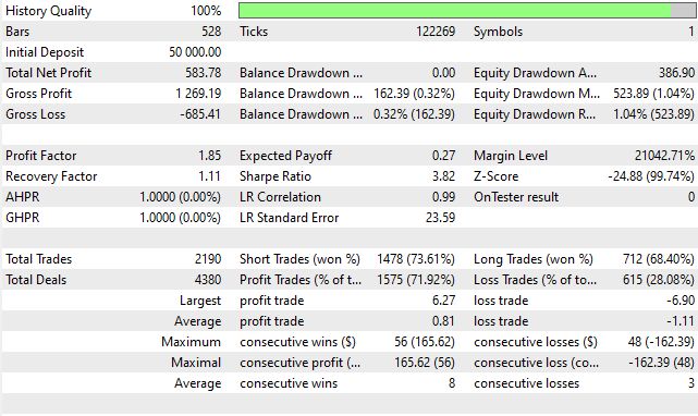
The Sharpe ratio is above 3, which means the strategy has a promising future.

Conclusion

A market-neutral strategy based on return distribution is a rare example of a mathematically sound approach that actually works in practice. Unlike most trading strategies based on technical analysis or attempts to predict the future, this method takes advantage of a fundamental property of markets — their statistical nature.

The key advantage of the strategy is its honesty. It does not promise outsized returns, nor does it claim to know where the price is headed. Instead, it acknowledges uncertainty and works with probabilities. The robot does not try to be right; it tries to be statistically profitable. The difference is critical.

Practical implementation requires attention to detail. The code, which looks simple at first glance, contains many nuances: correct percentile calculation, weighting volumes by probability, expiration of an outdated grid, and handling edge cases. Each of these details is important. Miss just one, and the strategy will stop working or start losing money under certain market conditions.

It is important to understand the limitations. The strategy is not universal. It performs better in sideways, volatile markets and worse in strong trends. It requires sufficient liquidity and reasonable spreads. It is vulnerable to black swan events and sharp news-driven moves. Being aware of these limitations does not weaken the strategy; on the contrary, it allows you to use it correctly.

Parameter optimization is not a one-time task. Markets change, volatility rises and falls, and correlations shift. What worked three months ago might not work now. Regular review of the WindowBars, HistoryBars, and LotMultiplier parameters is necessary. Keep a log of changes and results. In six months, you will have an invaluable body of knowledge about how the strategy performs on your trading instrument.

The psychological aspect is underestimated. Even with a fully automated trading bot, you will be tempted to intervene. A drawdown equal to 20% of your profit can trigger the urge to stop the trading bot. A string of losing trades raises doubts about the strategy. A period without profits causes anxiety. That is normal. It is important to remember that a statistical advantage becomes apparent over hundreds of trades, not just dozens. If you cannot patiently weather drawdowns, this strategy isn't for you.

Capital and risk management are critical. The strategy can open 10–15 positions simultaneously in various combinations. Make sure your deposit can handle it. The rule is simple: if you are trading 0.01 lots and a maximum of 10 positions with weights of up to 5x, you will need a minimum deposit of $500–$1,000 for EUR/USD. Any less than that, and you risk a margin call if things go wrong.

Backtesting is essential, but it is not enough. A strategy will produce different results in backtesting and in live trading. Slippage, execution delays, requotes, and spread fluctuations during news events — none of these occur in an ideal backtest. Be sure to conduct forward testing on a demo account for at least two to three months. Only then should you switch to a live account with minimum lot sizes.

Document everything. Every grid placement, every expiration, every parameter change, every drawdown, and every recovery. A year from now, this data will help you identify patterns that are invisible in the moment. You will see that the strategy performs very well on Tuesdays and Thursdays, but worse on Fridays. That July is consistently worse than March. That a period of profitability follows a sharp increase in volatility. This knowledge is invaluable.

A strategy based on return distribution is an instrument, not magic. Like any instrument, it requires understanding, configuration, monitoring, and adaptation. In the right hands, with the right expectations, it provides a consistent mathematical advantage. That is all it takes to achieve long-term profitability in the markets. Not the Holy Grail, not a get-rich-quick scheme, but simply honest statistical arbitrage that works because it uses the actual properties of price rather than trying to predict the unpredictable.