Self Optimizing Expert Advisors in MQL5 (Part 9): Double Moving Average Crossover

In our series of articles, we have explored multiple perspectives on how to reduce lag in the classical moving average crossover trading strategy.

Our initial attempts involved using statistical modeling tools to forecast moving average crossovers in advance. We made progress in this direction and found that, under the right market conditions, forecasting moving average crossovers can be more accurate than forecasting price directly. From there, we discovered yet another method to further reduce lag. This approach involves fixing the periods of the two moving averages so they share a common value, and instead generating crossovers by applying one moving average to the opening price and the other to the closing price. This alternative system proved effective, allowing us to reduce lag further without relying on advanced modeling tools—just by using the same period and varying the applied price of the two indicators.

In this discussion, we explore yet another unique approach that we have not considered before. As with most problems in life and mathematics, there is more than one way to tackle an issue, and each solution comes with its own set of advantages and disadvantages. By weighing these alternatives, we aim to understand how much control we can exert over lag in the system.

Here, we will attempt what I refer to as a double moving average crossover strategy. As shown in Figure 1, the classical moving average crossover strategy is typically used on a single timeframe with two moving averages of different periods. Unlike our previous discussion—where both moving averages shared a fixed period—this time we revert slightly to the classical approach, allowing the two indicators to use different periods.

The problem with this original form is that confirmation for entry signals often arrives late—after the move has already begun—leading to delayed entries or missed opportunities. 

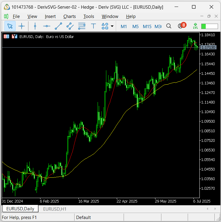
Figure 1: Visualizing our moving average crossover strategy on the daily time frame.

What we propose here is not entirely new. In fact, discretionary or human traders have long used similar logic. The core idea is to first observe crossover patterns on a higher timeframe (e.g., the daily chart as shown in Figure 1). However, we don’t immediately act on these signals. Instead, once we see a crossover on the higher timeframe, we drill down to a lower timeframe—such as the M30 shown in Figure 2—and look for crossover patterns that correspond with what we observed on the higher timeframe.

Human traders have often said, “Trade in line with the higher timeframe.” In most of our algorithmic trading discussions, we apply and trade a strategy on the same timeframe. Today, however, we apply the strategy twice—once on a higher timeframe and again on a lower one. The higher timeframe provides a directional bias for the day, while the lower timeframe is where we look for entry signals that align with that bias. This is the essence of our double crossover strategy. By first establishing a bias on a higher time frame and then searching for opportunities to trade in line with it on a lower time frame, we hope to factor out the lag introduced by signals generated by the higher time frame.

Now that we’re aligned in our understanding, we can begin implementing the strategy to determine whether it holds merit. Before diving into the code, it’s clear that this approach contains several moving parts we must consider carefully. One key question is, how do we define entry conditions? Suppose the higher timeframe shows a bullish crossover. We then have two options on the lower timeframe:

1. Contrarian Entry: Wait for a bearish crossover on the lower timeframe, then bet against it—believing that the lower timeframe will eventually realign with the bullish bias by the end of the day.
2. Trend-Following Entry: Simply wait for the lower timeframe to form a bullish crossover in the same direction as the higher timeframe bias.

These two options represent distinct ideologies for entering trades under this strategy. Exiting positions introduces even more complexity and variation, each with its own trade-offs. For instance, we might decide to close a position when the lower timeframe no longer aligns with the bias from the higher timeframe. Alternatively, we may only exit when the bias itself changes on the higher timeframe. So, if we start the day with a bullish signal on the daily chart, we hold our position until that higher timeframe flips to bearish.

As you can see, there are many ways to enter and exit trades using this method. Rather than relying on reasoning alone to determine the optimal combination, we must use a genetic optimizer. This will help us identify, from market data, which combination of these alternatives could be the most profitable.

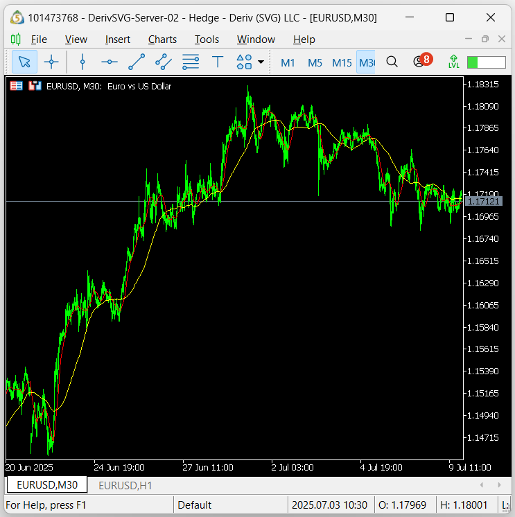
Figure 2: Visualizing our moving average crossover strategy on a lower timeframe, the M30. 

The first step we will take is to define a few system constants that must remain fixed throughout the development phase of our application. For simplicity, we will hold the timeframes constant: the daily chart will serve as a proxy of our higher timeframe, the M15 as our lower timeframe, and the H4 as the timeframe used to calculate our stop loss.

We may consider turning these system constants into tunable parameters that a genetic optimizer can leverage to ensure we achieve the best possible entries. However, to get us off the ground, we will keep these values fixed.

//+------------------------------------------------------------------+
//|                                             Double Crossover.mq5 |
//|                                  Copyright 2024, MetaQuotes Ltd. |
//|                                             https://www.mql5.com |
//+------------------------------------------------------------------+
#property copyright "Copyright 2024, MetaQuotes Ltd."
#property link      "https://www.mql5.com"
#property version   "1.00"

//+------------------------------------------------------------------+
//| System constants                                                 |
//+------------------------------------------------------------------+
//--- System time frames
#define TF_1            PERIOD_D1
#define TF_2            PERIOD_M15
#define TF_3            PERIOD_H4
#define LOT_MULTILPLE   1
    

We also need to define a set of custom enumerations to represent the different modes in which our strategy can operate. For example, the application can run in a trend-following mode or a mean-reverting mode, and a dedicated enumeration allows the user to switch between them. Similarly, we define another enumeration for specifying whether our closing conditions should be evaluated on the lower timeframe or the higher timeframe.

//+------------------------------------------------------------------+
//| Custom enumerations                                              |
//+------------------------------------------------------------------+
//--- What trading style should we follow when opening our positions, trend following or mean reverting?
enum STRATEGY_MODES  {
     TREND = 0,             //Trend Following Mode
     MEAN_REVERTING = 1     //Mean Reverting Mode
};

//--- Which time frame should we consult, when determining if we should close our position?
enum CLOSING_TIME_FRAME {
     HIGHER_TIME_CLOSE = 0, //Close on higher time frames
     LOWER_TIME_CLOSE = 1   //Close on lower time frames
};

Our input parameters are fairly straightforward. We will specify one period value on the higher timeframe and then define a gap between the first and second moving average periods. This design ensures that the genetic optimizer selects a gap of one or more—enforcing a non-zero difference between the periods by construction.

//+------------------------------------------------------------------+
//| Inputs                                                           |
//+------------------------------------------------------------------+
input group "Technical Indicators"
input int ma_1_period = 10;   //Higher Time Frame Period
input int ma_1_gap    = 20;   //Higher Time Frame Period Gap

input int ma_2_period = 10;   //Lower Time Frame Period
input int ma_2_gap    = 20;   //Lower Time Frame Period Gap

input group "Strategy Settings"
input STRATEGY_MODES     strategy_mode = 0;  //Strategy Operation Mode
input CLOSING_TIME_FRAME closing_tf    = 0;  //Strategy Closing Timeframe

The application will require only a moderate number of global variables, such as the technical indicators and instances used to keep track of current market prices.

//+------------------------------------------------------------------+
//| Global variables                                                 |
//+------------------------------------------------------------------+
int      ma_c_1_handle,ma_c_2_handle,ma_c_3_handle,ma_c_4_handle;
double   ma_c_1[],ma_c_2[],ma_c_3[],ma_c_4[];
double   volume_min;
double   bid,ask;
int      state;

The only external dependency required for this exercise is the Trade library, which we use to load and close positions as needed.

//+------------------------------------------------------------------+
//| Libraries                                                        |
//+------------------------------------------------------------------+
#include <Trade\Trade.mqh>
CTrade Trade;

Upon initialization, we will configure the technical indicators using the settings passed by the user. We will also reset the system state to -1, indicating no open positions, and record the minimum trading volume permitted on the market.

//+------------------------------------------------------------------+
//| Expert initialization function                                   |
//+------------------------------------------------------------------+
int OnInit()
  {
//---
   volume_min     = SymbolInfoDouble(Symbol(),SYMBOL_VOLUME_MIN);
   ma_c_2_handle  = iMA(Symbol(),TF_1,ma_1_period,0,MODE_SMA,PRICE_CLOSE);
   ma_c_1_handle  = iMA(Symbol(),TF_1,(ma_1_period + ma_1_gap),0,MODE_SMA,PRICE_CLOSE);
   ma_c_4_handle  = iMA(Symbol(),TF_2,ma_2_period,0,MODE_SMA,PRICE_CLOSE);
   ma_c_3_handle  = iMA(Symbol(),TF_2,(ma_2_period + ma_2_gap),0,MODE_SMA,PRICE_CLOSE);
   state          = -1;
//---
   return(INIT_SUCCEEDED);
  }

If the application is no longer in use, we will release the technical indicators to free memory.

//+------------------------------------------------------------------+
//| Expert deinitialization function                                 |
//+------------------------------------------------------------------+
void OnDeinit(const int reason)
  {
//---
   IndicatorRelease(ma_c_1_handle);
   IndicatorRelease(ma_c_2_handle);
   IndicatorRelease(ma_c_3_handle);
   IndicatorRelease(ma_c_4_handle);
  }

When new price data is received, we check for a new candle on the lower timeframe (M15, in this case). If a new candle is detected, we proceed to update our internal system state.

//+------------------------------------------------------------------+
//| Expert tick function                                             |
//+------------------------------------------------------------------+
void OnTick()
  {
//---
   datetime current_time = iTime(Symbol(),TF_2,0);
   static datetime time_stamp;

   if(time_stamp != current_time)
     {
      time_stamp = current_time;
      update();
     }
  }
//+------------------------------------------------------------------+

One of the most important components is the function used to identify trading setups. This function accepts a parameter known as padding, which represents the stop-loss size for our positions. Padding is calculated by the parent function using historical range levels naturally. As a safety measure, the setup function first checks if our total open positions is zero to prevent overtrading.

If a bullish crossover occurs on the higher timeframe, and our strategy is in trend-following mode, the setup function searches for a matching bullish crossover on the lower timeframe. If we are operating in mean-reversion mode, it looks for the opposite crossover (i.e., bearish) and bets against it. The logic is mirrored for bearish entries: if a bearish crossover occurs on the higher timeframe, we look for a corresponding signal on the lower timeframe, depending on the selected mode.

//+------------------------------------------------------------------+
//| Find a trading signal                                            |
//+------------------------------------------------------------------+
void find_setup(double padding)
  {
   if(PositionsTotal() == 0)
     {
      //--- Reset the system state
      state = -1;

      //--- Bullish on the higher time frame
      if(ma_c_1[0] > ma_c_2[0])
        {
         //--- Trend following mode
         if((ma_c_3[0] > ma_c_4[0]) && (strategy_mode == 0))
           {
            Trade.Buy(volume_min,Symbol(),ask,(bid - padding),0,"");
            state = 1;
           }
         //--- Mean reverting mode
         if((ma_c_3[0] < ma_c_4[0]) && (strategy_mode == 1))
           {
            Trade.Buy(volume_min,Symbol(),ask,(bid - padding),0,"");
            state = 1;
           }
        }

      //--- Bearish on the higher time frame
      if(ma_c_1[0] < ma_c_2[0])
        {
         //--- Trend following mode
         if((ma_c_3[0] < ma_c_4[0]) && (strategy_mode == 0))
           {
            Trade.Sell(volume_min,Symbol(),bid,(ask + padding),0,"");
            state = 0;
           }
         //--- Mean reverting mode
         if((ma_c_3[0] > ma_c_4[0]) && (strategy_mode == 1))
           {
            Trade.Sell(volume_min,Symbol(),bid,(ask + padding),0,"");
            state = 0;
           }
        }
     }
  }

Once a position is opened, we call a separate position management function, which also operates in two distinct modes depending on whether we want to close trades based on the lower or the higher timeframe. The system state is updated when positions are opened, and this state determines trade direction. For example, if the state is zero, we opened a sell trade. If the first moving average is now above the second (indicating bullish momentum on the daily), and if we're managing exits based on the higher timeframe, we will close the position. Otherwise, if managing based on the lower timeframe, we wait for a crossover there. It is not immediately obvious which exit condition is more effective, so both options must be tested.

//+------------------------------------------------------------------+
//| Manage our open positions                                        |
//+------------------------------------------------------------------+
void manage_setup(void)
  {
   if(closing_tf == 0)
     {
      if((state ==0) && (ma_c_1[0] > ma_c_2[0]))
         Trade.PositionClose(Symbol());
      if((state ==1) && (ma_c_1[0] < ma_c_2[0]))
         Trade.PositionClose(Symbol());
     }

   else
      if(closing_tf == 1)
        {
         if((state ==0) && (ma_c_3[0] > ma_c_4[0]))
            Trade.PositionClose(Symbol());
         if((state ==1) && (ma_c_3[0] < ma_c_4[0]))
            Trade.PositionClose(Symbol());
        }
  }

Lastly, we need a function to update key system variables, such as the current bid and ask prices. We will also track the previous 10 high and low values occurring in the third timeframe—our risk timeframe. In this example, the risk timeframe is H4, which sits nicely between the M15 and the daily. This makes it a useful candidate for measuring market risk and setting stop losses that are neither too tight nor too far from the entry.

//+------------------------------------------------------------------+
//| Update our technical indicators and positions                    |
//+------------------------------------------------------------------+
void update(void)
  {
   
   //Update technical indicators and market readings
   CopyBuffer(ma_c_2_handle,0,0,1,ma_c_2);
   CopyBuffer(ma_c_1_handle,0,0,1,ma_c_1);
   CopyBuffer(ma_c_4_handle,0,0,1,ma_c_4);
   CopyBuffer(ma_c_3_handle,0,0,1,ma_c_3);
   bid = SymbolInfoDouble(Symbol(),SYMBOL_BID);
   ask = SymbolInfoDouble(Symbol(),SYMBOL_ASK);
   vector high = vector::Zeros(10);
   vector low = vector::Zeros(10);
   low.CopyRates(Symbol(),TF_3,COPY_RATES_LOW,0,10);
   high.CopyRates(Symbol(),TF_3,COPY_RATES_HIGH,0,10);
   vector var = high - low;
   double padding = var.Mean();

   //Find an open position
   if(PositionsTotal() == 0)
      find_setup(padding);

   //Manage our open positions
   else
      if(PositionsTotal() > 0)
         manage_setup();
  }
//+------------------------------------------------------------------+

For us to get started with our backtesting process, we must first select the expert advisor that we have just built together—the double crossover EX5. From there, we select the EURUSD symbol, the one-minute timeframe, and a backtest period running from January 2020 until this year—a five-year backtest. We’ll forward test using half of the data at hand to keep our results as realistic as possible. 

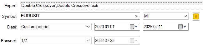
Figure 3: Selecting our trading application and our training dates.

To simulate real market conditions, we’ll set delays randomly and use real ticks as our modeling mode. Recall that our optimization procedure will use a fast, genetic-based algorithm.

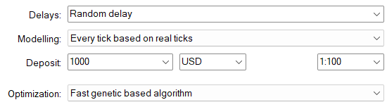
Figure 4: Selecting market simulation conditions.

Next, we must select the input parameters of our strategy that need to be adjusted, as previously discussed. These include the moving average crossover period and gap on both the higher and lower timeframes. Additionally, we’ll enable two operational modes for the strategy: trend-following and mean-reverting. Lastly, the strategy can be configured to close positions based on either the higher or lower timeframe. All of these settings are what our genetic optimizer will search through to help us select the most appropriate parameters.

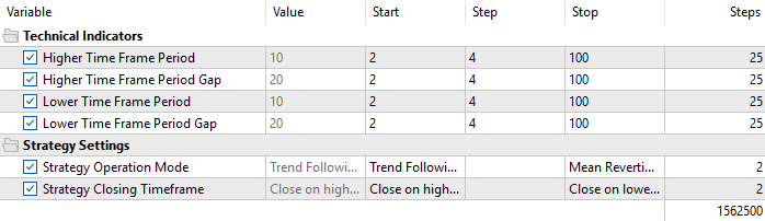
Figure 5: Selecting the strategy parameters to be adjusted by our genetic optimizer.

The backtest results appear encouraging. As seen in our optimization results, most of our strategies were profitable—especially in mean-reverting mode. However, when considering the forward test results, we find that most profitable strategies operated in trend-following mode rather than mean-reverting, as observed in the backtest.

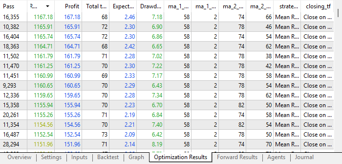
Figure 6: The back test results from our initial test.

More concerning is that when we take a closer look at the forward results, none of the backtest strategies match the forward test results. That is, almost none of the strategies that performed well in the forward test were also profitable in the backtest.

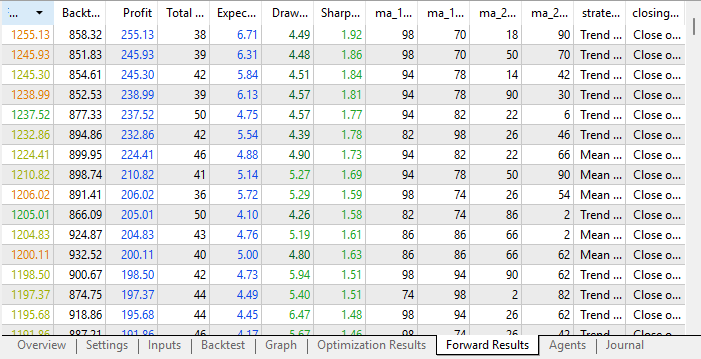
Figure 7: The forward results from our initial test indicate that most of our strategies were not stable across both tests.

I had to manually filter through the forward results to find strategy settings that were profitable in both tests. This is what we look for as a sign of stability—that a strategy should be profitable across both the backtest and forward test. Seeing that only a handful of configurations met this standard encouraged me to try additional refinements.

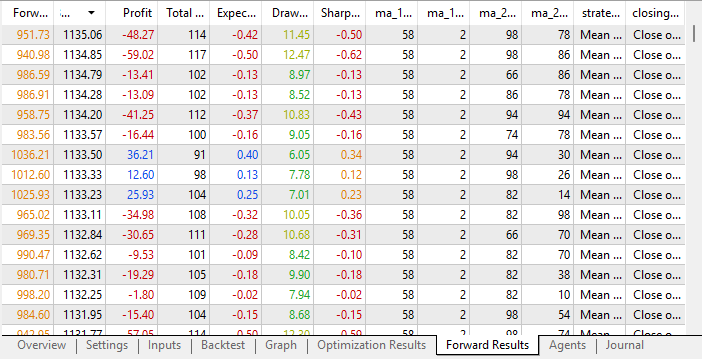
Figure 8: Only a handful of the strategies that were produced by our genetic optimizer were profitable across both tests. This is not a good indicator. 

Further Improvements

One strong case for improving the strategy is to allow the genetic optimizer to control the timeframe used to calculate stop loss and risk parameters. Additionally, we’ll let the optimizer decide how many historical bars should be used in the stop loss calculation. In our first attempt, we had assumed that 10 H4 bars would be sufficient. But now, we’ll allow the optimizer to adjust this setting and test whether this change improves performance.

//+------------------------------------------------------------------+
//| Inputs                                                           |
//+------------------------------------------------------------------+
input group "Money Management Settings"
input ENUM_TIMEFRAMES TF_3 =    PERIOD_H4; //Risk Time Frame
input int HISTORICAL_BARS  =           10; //Historical bars for risk calculation

We must also introduce changes to the code. In the previous version, the update method handled the calculation of padding for each position. In this new version, a separate function will handle padding, as we now want the stop loss to trail and follow winning positions.

//+------------------------------------------------------------------+
//| Get the stop loss size to use                                    |
//+------------------------------------------------------------------+
double get_padding(void)
  {
   vector high = vector::Zeros(10);
   vector low = vector::Zeros(10);
   low.CopyRates(Symbol(),TF_3,COPY_RATES_LOW,0,HISTORICAL_BARS);
   high.CopyRates(Symbol(),TF_3,COPY_RATES_HIGH,0,HISTORICAL_BARS);
   vector var = high - low;
   double padding = var.Mean();
   return(padding);
  }

The update method will change accordingly. Padding will now be calculated using the get_padding method. The part of the update method that initially identified positions will now call a function responsible for finding our setup and another method for managing open positions. 

//+------------------------------------------------------------------+
//| Update our technical indicators and positions                    |
//+------------------------------------------------------------------+
void update(void)
  {

//Update technical indicators and market readings
   CopyBuffer(ma_c_2_handle,0,0,1,ma_c_2);
   CopyBuffer(ma_c_1_handle,0,0,1,ma_c_1);
   CopyBuffer(ma_c_4_handle,0,0,1,ma_c_4);
   CopyBuffer(ma_c_3_handle,0,0,1,ma_c_3);
   bid = SymbolInfoDouble(Symbol(),SYMBOL_BID);
   ask = SymbolInfoDouble(Symbol(),SYMBOL_ASK);
   double padding = get_padding();

//Find an open position
   if(PositionsTotal() == 0)
      find_setup(padding);

//Manage our open positions
   else
      if(PositionsTotal() > 0)
         manage_setup();
  }
//+------------------------------------------------------------------+

The method that manages positions will always check if the new suggested stop loss value is more profitable than the current one. If so, it updates the stop loss; otherwise, it keeps the current value.

//+------------------------------------------------------------------+
//| Manage our open positions                                        |
//+------------------------------------------------------------------+
void manage_setup(void)
  {
  //Does the position exist?
  if(PositionSelect(Symbol()))
   {
      //Get the current stop loss
      double current_sl = PositionGetDouble(POSITION_SL);
      double padding = get_padding();
      double new_sl;
      
   
      //Sell position
      if((state == 0))
      {
         new_sl = (ask + padding);
         
         if(new_sl < current_sl) Trade.PositionModify(Symbol(),new_sl,0);
      }

      //Buy position
      if((state == 1))
      {
         new_sl = (bid - padding);
         
         if(new_sl > current_sl) Trade.PositionModify(Symbol(),new_sl,0);
      }
  
  
   if(closing_tf == 0)
     {
      if((state ==0) && (ma_c_1[0] > ma_c_2[0]))
         Trade.PositionClose(Symbol());
      if((state ==1) && (ma_c_1[0] < ma_c_2[0]))
         Trade.PositionClose(Symbol());
     }

   else
      if(closing_tf == 1)
        {
         if((state ==0) && (ma_c_3[0] > ma_c_4[0]))
            Trade.PositionClose(Symbol());
         if((state ==1) && (ma_c_3[0] < ma_c_4[0]))
            Trade.PositionClose(Symbol());
        }
   }
  }

To conduct our tests, I selected one configuration that had been profitable in both the backtest and forward test, then held other settings fixed while allowing the genetic optimizer to search for better risk parameter settings. 

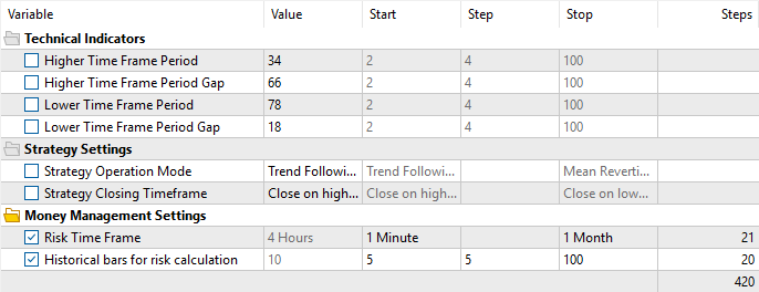
Figure 9: Trying to improve our initial results. Even though we permitted the genetic optimizer to control the risk settings, our new results were not yet profitable across both tests.

Unfortunately, we ran yet into the same problem all over again. And when we were optimizing our risk parameter settings, our application was only profitable in the forward test and failed to be profitable in the backtest. 

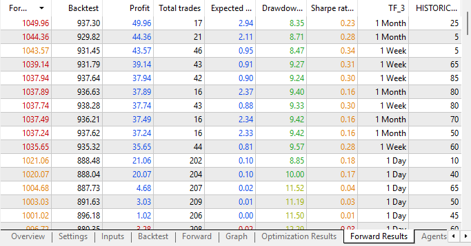
Figure 10: Our new results were still not yet profitable across both tests. 

Conclusion

We’ve learned a lot from this exercise. With our double moving average crossover strategy, we’ve observed that we can indeed control the amount of lag in the strategy—though the consequences of those changes aren’t always immediately clear. We may want to reconsider rerunning the optimization with all available parameters simultaneously. It’s possible that adjusting one parameter while holding others fixed is not the optimal approach. Searching all parameters at once may yield more stable results.

In our follow-up discussion, after re-performing a full optimization sweep, we’ll build statistical models based on the most profitable configurations. This may help us reduce lag further. For now, however, we are off to a strong start. Remember that optimization offers us no guarantees, and AI is no substitute for hardworking developers. We must repeat our optimization procedure until our genetic optimizer can offer us batches of strategies that are profitable across both tests, otherwise the optimization is likely premature.