Neural Networks in Trading: Skill Hierarchy for Adaptive Agent Behavior (Final Part)

Introduction

In the previous article, we examined the theoretical foundations of the HiSSD framework (Hierarchical and Separate Skill Discovery), a modern approach to offline training of multi-agent systems capable of operating in complex and highly dynamic environments. This framework enables agents to learn effective interaction patterns and adapt to changing conditions. Initially, HiSSD was tested in simulated environments; however, its architecture and design principles make it particularly relevant for financial markets, where conditions can shift dramatically within seconds and intelligent trading agents are required to respond rapidly and in a coordinated manner.

One of the key advantages of HiSSD is its high degree of adaptability. In trading scenarios, where economic indicators, market participant behavior, or news events can abruptly reshape the market landscape, agents trained under HiSSD can adjust instantly without full retraining. This is enabled by a two-level skill decomposition architecture: common and task-specific skills. Common skills represent behavioral patterns applicable across a wide range of situations — for example, trend recognition or risk assessment. Task-specific skills, in turn, govern behavior in unique or highly specialized conditions. This dual-layer structure allows HiSSD agents to remain stable and effective regardless of changing market regimes.

Another strong aspect of HiSSD is its scalability. Financial markets represent a multi-agent system. Every participant here — whether a human trader, algorithmic system, or large market maker — influences overall dynamics. In such environments, it is essential to scale the system without breaking its internal consistency. HiSSD proposes a hierarchical architecture where each agent can coordinate its behavior with others through shared control modules. This is especially useful when designing complex strategies. In practice, it enables the construction of more robust and resilient trading systems.

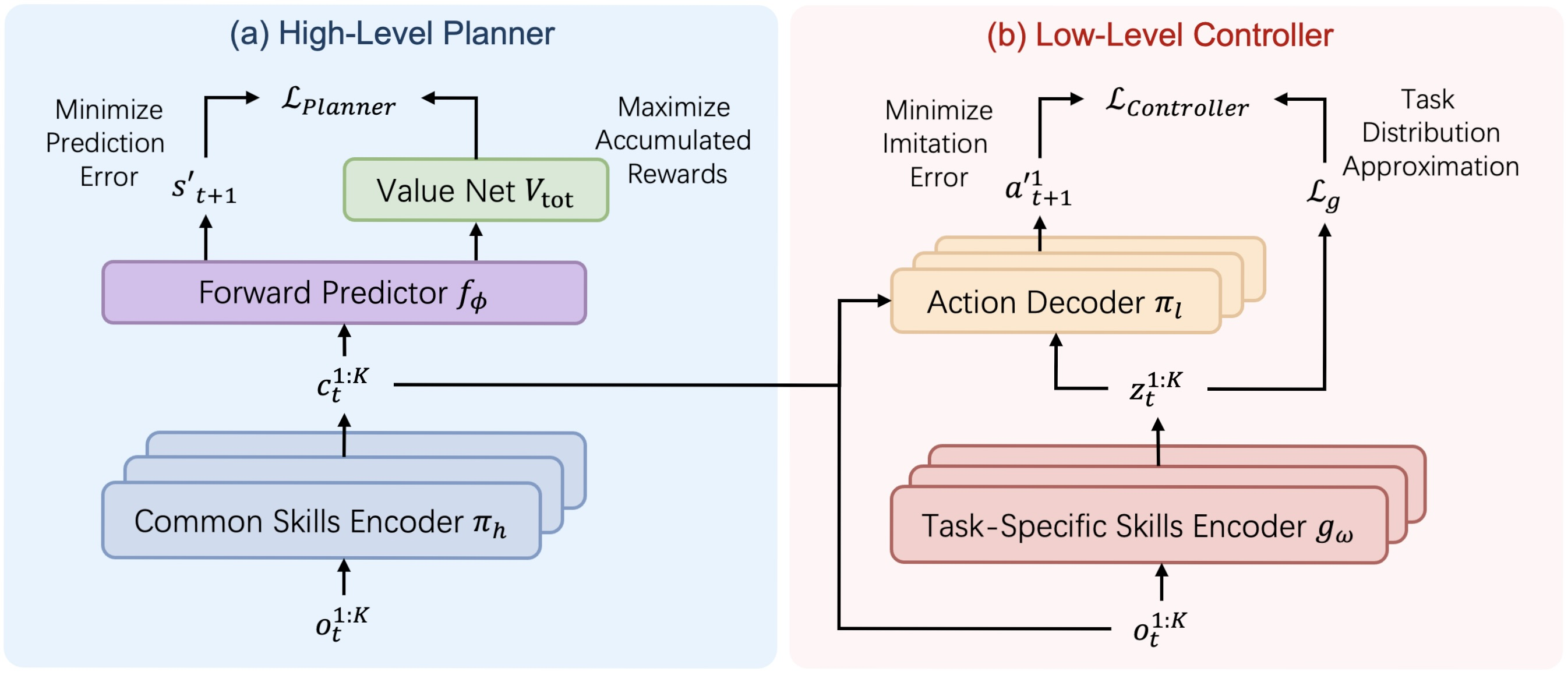
A visualization of the HiSSD framework architecture created by the authors is shown below.

In the practical section of the previous article, we began implementing our interpretation of the framework proposed by the authors using MQL5. In particular, we introduced a version of a universal skill encoder implemented within the CNeuronSkillsEncoder class. In this article, we continue this work and bring it to completion, including testing the effectiveness of the implemented approach on real historical data.

Before proceeding further, let us once again review the structure of the HiSSD framework. It consists of two major components: the Planner and the Controller.

The Planner follows a linear information flow. Raw input data passes through a common skill encoder and is then fed into a prediction module responsible for forecasting future states and expected value. This architecture can be implemented using existing tools as a standard linear model.

The Controller is more complex in terms of organization. It includes an action decoder for agents that receives input from three sources: local agent observations, common skills, and task-specific skills generated by different encoders. This structure motivates us to implement the Controller as a separate dedicated object.

Controller Object

The next step in our implementation is the construction of the Controller object, encapsulated in the CNeuronHiSSDLowLevelControler class.

class CNeuronHiSSDLowLevelControler:  public CNeuronConvOCL
  {
protected:
   uint                       iTaskSkills;
   uint                       iCommonSkills;
   //---
   CNeuronSkillsEncoder       cTaskSpecificSkillsEncoder;
   CNeuronTransposeOCL        cTranspose;
   CNeuronBaseOCL             cObservAndSkillsConcat;
   CNeuronBatchNormOCL        cNormalizarion;
   CNeuronConvOCL             cActionDecoder[2];
   //---
   virtual bool               feedForward(CNeuronBaseOCL *NeuronOCL) override { return false; }
   virtual bool               feedForward(CNeuronBaseOCL *NeuronOCL, CBufferFloat *SecondInput) override;
   virtual bool               updateInputWeights(CNeuronBaseOCL *NeuronOCL) override { return false; }
   virtual bool               updateInputWeights(CNeuronBaseOCL *NeuronOCL, CBufferFloat *second) override;
   virtual bool               calcInputGradients(CNeuronBaseOCL *prevLayer) override { return false; }
   virtual bool               calcInputGradients(CNeuronBaseOCL *NeuronOCL,
                                                 CBufferFloat *SecondInput,
                                                 CBufferFloat *SecondGradient,
                                                 ENUM_ACTIVATION SecondActivation = None
                                                ) override;

public:
                              CNeuronHiSSDLowLevelControler(void) {};
                             ~CNeuronHiSSDLowLevelControler(void) {};
   //---
   virtual bool               Init(uint numOutputs, uint myIndex, COpenCLMy *open_cl,
                                   uint time_step, uint variables,
                                   uint task_skills, uint common_skills, uint n_actions,
                                   uint window, uint step, uint window_key, uint heads,
                                   ENUM_OPTIMIZATION optimization_type, uint batch);
   //---
   virtual int                Type(void) override const   {  return defNeuronHiSSDLowLevelControler;   }
   //---
   virtual bool               Save(int const file_handle) override;
   virtual bool               Load(int const file_handle) override;
   //---
   virtual bool               WeightsUpdate(CNeuronBaseOCL *source, float tau) override;
   virtual void               SetOpenCL(COpenCLMy *obj) override;
  };

It is important to note that the agent action decoder within the HiSSD Controller assumes parallel execution of multiple independent agents. This functionality can be implemented using sequential convolutional layers. Since the decoder is positioned at the output stage of the module, the functionality of the final decoding layer can be delegated to the parent class. For this reason, we chose a convolutional layer object as the base class for the Controller module.

In the structure of the new object, we define several internal components whose detailed functionality will be discussed during the implementation of feed-forward and backpropagation algorithms. At this stage, we simply note their static declaration, which allows the constructor and destructor to remain empty. Initialization of all internal objects, including inherited ones, is performed in the Init method.

As usual, the initialization method receives a set of constants that uniquely define the architecture of the required object.

bool CNeuronHiSSDLowLevelControler::Init(uint numOutputs, uint myIndex, COpenCLMy *open_cl,
                                         uint time_step, uint variables, uint task_skills,
                                         uint common_skills, uint n_actions, uint window,
                                         uint step, uint window_key, uint heads,
                                         ENUM_OPTIMIZATION optimization_type, uint batch)
  {
   if(!CNeuronConvOCL::Init(numOutputs, myIndex, open_cl, window_key, window_key,
                            n_actions, 1, variables, optimization_type, batch))
      return false;
   SetActivationFunction(SIGMOID);

Within the method body, we first call the corresponding parent class method, as is our standard practice. Here, several key aspects must be highlighted.

First, we intend to use the parent class functionality as the final layer of the agent action decoder. Therefore, the input to the parent class methods will consist of the processed outputs of internal decoder components. The decoder is expected to organize parallel information flows that form the "consciousness" of individual agents. Consequently, the analyzed data window size and stride of the convolutional layer are set equal to the dimensionality of the internal information vector of a single agent.

On the output side, we expect to obtain a tensor of agent actions. Therefore, the number of convolutional filters corresponds to the dimensionality of the action vector of a single agent.

There's one more thing here. To ensure fully independent learning for each agent, we must assign unique weight parameters. This is achieved by setting the input sequence dimension to one and moving the number of trainable agents into the parameter defining the number of unit sequences. This simple technique allows us to implement fully parallel operation of an arbitrary number of independent agents.

Next, we proceed to initialize the internal objects declared in the class structure. As mentioned earlier, initialization of inherited components is handled by the parent class method, which has already been called.

The first component to initialize is the task-specific skills encoder, implemented using the universal skill encoder developed in the previous article.

int index = 0;
if(!cTaskSpecificSkillsEncoder.Init(0, index, OpenCL, time_step, variables, task_skills,
                                    window, step, window_key, heads, optimization, iBatch))
   return false;
cTaskSpecificSkillsEncoder.SetActivationFunction(None);

We then store the necessary architectural constants.

iTaskSkills = task_skills;
iCommonSkills = MathMax(common_skills, 1);

Note that the dimensionality of specific skills is preserved as is, while common skills are assigned a minimal valid value. This is straightforward. We previously passed the dimension of task-specific skills in the parameters of the encoder initialization method. And successful execution of this method confirms the validity of the obtained value. However, common skill tensors are provided by the Planner, which is a separate object and even a separate model in this implementation. Therefore, only a minimal acceptable constraint can be defined here.

Next, we proceed to constructing the agent action decoder. The authors of the HiSSD framework propose three input sources for the decoder:

• local agent observations
• common skills
• task-specific skills

As noted earlier, common skills are expected from a separate model via an auxiliary information flow. Specific skills are generated by the encoder based on local observations from the main input stream. Thus, all required data is already available. It only needs to be merged into a unified structure.

It is important to emphasize that each agent must receive its own unique data representation. Therefore, correct concatenation must be ensured. Skill tensors are represented as an abstract matrix where each row corresponds to the skill vector of an individual agent. Row-wise concatenation yields the desired matrix suitable for parallel processing of independent information flows using the functionality of convolutional layers.

Local observations are handled slightly differently. As previously discussed, the input is assumed to be a multimodal time series. Each agent in it processes its own univariate sequence. Before concatenation with skill tensors, the observation matrix must be transposed into a format suitable for processing univariate sequences.

index++;
if(!cTranspose.Init(0, index, OpenCL, time_step, variables, optimization, iBatch))
   return false;

We then determine the dimensionality of a single agent's input vector and initialize a buffer for the concatenated tensor.

uint window_size = (time_step + iTaskSkills + iCommonSkills);
index++;
if(!cObservAndSkillsConcat.Init(0, index, OpenCL, window_size * iVariables,
                                optimization, iBatch))
   return false;
cObservAndSkillsConcat.SetActivationFunction(None);

It is worth reiterating that data originates from three sources. To ensure compatibility, we apply batch normalization to harmonize their distributions.

index++;
if(!cNormalizarion.Init(0, index, OpenCL, cObservAndSkillsConcat.Neurons(),
                        iBatch, optimization))
   return false;
cNormalizarion.SetActivationFunction(None);

After completing data preparation, we proceed to constructing the neural layers of the action decoder. Here we create a loop, in whose body we initialize the decoder's convolutional layers. The implementation principles were described during initialization of the parent class.

   for(uint i = 0; i < cActionDecoder.Size(); i++)
     {
      index++;
      if(!cActionDecoder[i].Init(0, index, OpenCL, window_size, window_size, window_key,
                                 1, iVariables, optimization, iBatch))
         return false;
      cActionDecoder[i].SetActivationFunction(SoftPlus);
      window_size = window_key;
     }
//---
   return true;
  }

The method concludes by returning the logical result of the operation to the calling program.

Next, we move on to constructing the feed-forward pass algorithm in the feedForward method. As mentioned earlier, we operate with two data sources. Via the main stream, we receive a multimodal time series describing the environment state, and via an auxiliary stream we receive a tensor of common skills.

bool CNeuronHiSSDLowLevelControler::feedForward(CNeuronBaseOCL *NeuronOCL, CBufferFloat *SecondInput)
  {
   if(!SecondInput)
      return false;

First, we verify the validity of the pointer to the common skills tensor. At the same time, we do not explicitly validate the main input pointer. Instead, it is directly passed to the relevant method of the task-specific skills encoder, which contains its own control point.

if(!cTaskSpecificSkillsEncoder.FeedForward(NeuronOCL))
   return false;

After generating the task-specific skills tensor, we transpose the environmental observation tensor and concatenate it row-wise with both skill matrices (common and task-specific).

if(!cTranspose.FeedForward(NeuronOCL))
   return false;
if(!Concat(cTranspose.getOutput(), cTaskSpecificSkillsEncoder.getOutput(), SecondInput,
           cObservAndSkillsConcat.getOutput(), cTranspose.GetCount(),
           iTaskSkills, iCommonSkills, iVariables))
   return false;

The resulting data is normalized and passed through the three-layer agent action decoder, producing a concatenated tensor of actions for all agents.

   if(!cNormalizarion.FeedForward(cObservAndSkillsConcat.AsObject()))
      return false;
   CNeuronBaseOCL *neuron = cNormalizarion.AsObject();
   for(uint i = 0; i < cActionDecoder.Size(); i++)
     {
      if(!cActionDecoder[i].FeedForward(neuron))
         return false;
      neuron = cActionDecoder[i].AsObject();
     }
//---
   return CNeuronConvOCL::feedforward(neuron);
  }

The method concludes by returning the logical result of the operation to the calling program.

We now proceed to the backpropagation process. It is divided into two stages:

• Distribution of error gradients among all participating components according to their contribution to the final model output
• Optimization of model parameters to reduce the error

The first stage is implemented in the calcInputGradients method. This method receives pointers to the input data streams and corresponding error gradients. We immediately validate these pointers.

bool CNeuronHiSSDLowLevelControler::calcInputGradients(CNeuronBaseOCL *NeuronOCL,
                                                       CBufferFloat *SecondInput,
                                                       CBufferFloat *SecondGradient,
                                                       ENUM_ACTIVATION SecondActivation = -1)
  {
   if(!NeuronOCL || !SecondGradient)
      return false;

Gradient propagation follows the same structure as the feed-forward pass, but in reverse order. The feed-forward pass ends with the action decoder. Therefore, backpropagation begins there by iterating through convolutional layers in reverse.

   uint total = cActionDecoder.Size();
   if(total <= 0)
      return false;
   CObject *neuron = cActionDecoder[total - 1].AsObject();
//---
   if(!CNeuronConvOCL::calcInputGradients(neuron))
      return false;
   for(int i = int(total - 2); i >= 0; i--)
     {
      if(!cActionDecoder[i].calcHiddenGradients(neuron))
         return false;
      neuron = cActionDecoder[i].AsObject();
     }

The resulting gradients are passed through a normalization layer down to the level of the concatenated three-source tensor.

if(!cNormalizarion.calcHiddenGradients(neuron))
   return false;
if(!cObservAndSkillsConcat.calcHiddenGradients(cNormalizarion.AsObject()))
   return false;

We then distribute the error gradients back into the three original streams by deconcatenating the data.

if(!DeConcat(cTranspose.getGradient(), cTaskSpecificSkillsEncoder.getGradient(), SecondGradient,
             cObservAndSkillsConcat.getGradient(), cTranspose.GetCount(),
             iTaskSkills, iCommonSkills, iVariables))
   return false;

It is important to note that each data stream may have its own activation function. Therefore, we check for activation layers in all information streams and, if necessary, adjust gradients using the corresponding derivatives.

if(SecondActivation != None)
  {
   if(!DeActivation(SecondInput, SecondGradient, SecondGradient, SecondActivation))
      return false;
  }
if(NeuronOCL.Activation() != None)
  {
   if(!DeActivation(cTranspose.getOutput(), cTranspose.getGradient(),
                    cTranspose.getGradient(), NeuronOCL.Activation()))
      return false;
  }
if(cTaskSpecificSkillsEncoder.Activation() != None)
  {
   if(!DeActivation(cTaskSpecificSkillsEncoder.getOutput(), cTaskSpecificSkillsEncoder.getGradient(),
                    cTaskSpecificSkillsEncoder.getGradient(), cTaskSpecificSkillsEncoder.Activation()))
      return false;
  }

At this stage, the gradient has been fully propagated back into the auxiliary data stream, which can now be considered complete. The remaining task is to aggregate gradients affecting the main input stream from both auxiliary and primary paths. We first pass data through the task-specific skills encoder.

if(!NeuronOCL.calcHiddenGradients(cTaskSpecificSkillsEncoder.AsObject()))
   return false;

We then substitute the gradient buffer pointer of the main input stream and propagate gradients through the second stream originating from the transposition module.

   CBufferFloat *temp = NeuronOCL.getGradient();
   if(!NeuronOCL.SetGradient(cTranspose.getPrevOutput(), false) ||
      !NeuronOCL.calcHiddenGradients(cTranspose.AsObject()) ||
      !SumAndNormilize(temp, NeuronOCL.getGradient(), temp, iVariables, false, 0, 0, 0, 1) ||
      !NeuronOCL.SetGradient(temp, false))
      return false;
//---
   return true;
  }

Finally, gradients from both streams are summed, and all buffer pointers are restored to their original state.

The method concludes by returning the execution result to the caller.

This completes the description of the Controller implementation in our interpretation of the HiSSD framework. The full source code of the new object and its methods is provided in the attachments for independent review.

Model Architecture

After completing the construction of the individual components of the HiSSD framework, we proceed to describe the architecture of the trainable models. It is important to note that we intend to train four models in total.

The first model is the Environmental State Encoder, which in this context plays the role of the Planner in the HiSSD framework. We plan to train it in a supervised learning regime. From the observed state of the environment, it generates the agents' common skills. Based on these skills, it is then used to describe future environmental states over a specified planning horizon.

Here, one may observe a deviation from the original formulation of the HiSSD, which considers only a single-step prediction of the next state. However, our goal is to develop a policy capable of opening positions and holding them over time, which requires deeper analysis and longer-horizon planning.

The second model is the Controller, which analyzes the current state of the environment and produces a tensor of actions for multiple agents.

The third model is the Manager (Actor). In our implementation, this model analyzes account state, evaluates the trading actions proposed by the Controller agents, and ultimately decides whether to execute a trade.

The fourth model is a predictive network that estimates the probability of the direction of the upcoming price movement.

The architecture of all trainable models is defined in the CreateDescriptions method.

bool CreateDescriptions(CArrayObj *&encoder, 
                        CArrayObj *&task, 
                        CArrayObj *&actor, 
                        CArrayObj *&probability)
  {
//---
   CLayerDescription *descr;
//---
   if(!encoder)
     {
      encoder = new CArrayObj();
      if(!encoder)
         return false;
     }
   if(!task)
     {
      task = new CArrayObj();
      if(!task)
         return false;
     }
   if(!actor)
     {
      actor = new CArrayObj();
      if(!actor)
         return false;
     }
   if(!probability)
     {
      probability = new CArrayObj();
      if(!probability)
         return false;
     }

The method receives pointers to four dynamic arrays used to store architectural descriptions of the respective models. All pointers are validated, and if necessary, new instances of the corresponding objects are created.

We begin by describing the architecture of the Environmental State Encoder. As usual, the model starts with a fully connected layer of sufficient size to embed the raw input data.

//--- Encoder
   encoder.Clear();
//--- Input layer
   if(!(descr = new CLayerDescription()))
      return false;
   descr.type = defNeuronBaseOCL;
   int prev_count = descr.count = (HistoryBars * BarDescr);
   descr.activation = None;
   descr.optimization = ADAM;
   if(!encoder.Add(descr))
     {
      delete descr;
      return false;
     }

The model receives unprocessed environmental observations, which are first standardized using a batch normalization layer.

//--- layer 1
   if(!(descr = new CLayerDescription()))
      return false;
   descr.type = defNeuronBatchNormOCL;
   descr.count = prev_count;
   descr.batch = 1e4;
   descr.activation = None;
   descr.optimization = ADAM;
   if(!encoder.Add(descr))
     {
      delete descr;
      return false;
     }

This is followed by a universal skill encoder, which in this configuration is responsible for generating the tensor of common skills.

//--- layer 2
   if(!(descr = new CLayerDescription()))
      return false;
   descr.type = defNeuronSkillsEncoder;
   descr.count = HistoryBars;
     {
      int temp[] = {BarDescr, NSkills, 4};   // Variables, Common Skills, Heads
      if(ArrayCopy(descr.windows, temp) < (int)temp.Size())
         return false;
     }
   descr.window = 8;
   descr.step = 1;
   descr.window_out = 32;
   prev_count = descr.windows[0];
   int prev_out = descr.windows[1];
   descr.batch = 1e4;
   descr.optimization = ADAM;
   descr.activation = None;
   if(!encoder.Add(descr))
     {
      delete descr;
      return false;
     }

Next, two convolutional layers are applied to predict the future evolution of individual unit sequences within the multimodal time series, conditioned on the common skill tensor.

//--- layer 3
   if(!(descr = new CLayerDescription()))
      return false;
   descr.type = defNeuronConvOCL;
   descr.count = 1;
   descr.window = prev_out;
   descr.step = prev_out;
   prev_out=descr.window_out = 4*NForecast;
   descr.layers = prev_count;
   descr.activation = SoftPlus;
   if(!encoder.Add(descr))
     {
      delete descr;
      return false;
     }
//--- layer 4
   if(!(descr = new CLayerDescription()))
      return false;
   descr.type = defNeuronConvOCL;
   descr.count = 1;
   descr.window = prev_out;
   descr.step = prev_out;
   prev_out=descr.window_out = NForecast;
   descr.layers = prev_count;
   descr.activation = TANH;
   if(!encoder.Add(descr))
     {
      delete descr;
      return false;
     }

It is important to emphasize that the predictive behavior of each unit sequence is constructed from the common skill vector of a single agent, over a defined planning horizon. As a result, the output of this planning block differs from a conventional multimodal time series representation. To restore a consistent format, the data must be transposed.

//--- layer 5
   if(!(descr = new CLayerDescription()))
      return false;
   descr.type = defNeuronTransposeOCL;
   descr.count = prev_count;
   descr.window = prev_out;
   descr.activation = None;
   if(!encoder.Add(descr))
     {
      delete descr;
      return false;
     }

Afterward, the transformed representation is returned to the original distribution space via inverse normalization.

//--- layer 6
   if(!(descr = new CLayerDescription()))
      return false;
   descr.type = defNeuronRevInDenormOCL;
   descr.count = prev_count*prev_out;
   descr.layers = 1;
   descr.activation = None;
   if(!encoder.Add(descr))
     {
      delete descr;
      return false;
     }

This completes the architecture of the Environmental State Encoder. Before moving on, we store the latent representation object containing the output common skill tensor.

//--- Latent
   CLayerDescription *latent = encoder.At(LatentLayer);
   if(!latent)
      return false;

The second model, as mentioned above, is the Controller. It generates task-specific agent skills based on the same environmental state representation. Therefore, we reuse the first two layers from the previous model.

//--- Task
   task.Clear();
//--- Input layer
   if(!task.Add(encoder.At(0)))
     {
      return false;
     }
//--- layer 1
   if(!task.Add(encoder.At(1)))
     {
      return false;
     }

The model is then completed by the previously constructed Controller module.

//--- layer 2
   if(!(descr = new CLayerDescription()))
      return false;
   descr.type = defNeuronHiSSDLowLevelControler;
   descr.count = HistoryBars;
     {
      int temp[] = {latent.windows[0], // Variables
                    NSkills,           // Task Skills
                    latent.windows[1], // Common Skills
                    NActions,          // Action Space
                    4};                // Heads
      if(ArrayCopy(descr.windows, temp) < (int)temp.Size())
         return false;
     }
   descr.window = 8;
   descr.step = 1;
   descr.window_out = 32;
   prev_count = descr.windows[0];
   prev_out = descr.windows[3];
   descr.batch = 1e4;
   descr.optimization = ADAM;
   descr.activation = SIGMOID;
   if(!task.Add(descr))
     {
      delete descr;
      return false;
     }

The third model, the higher-level Manager, receives account state vectors as input. A fully connected layer is used to embed this information.

//--- Actor
   actor.Clear();
//--- Input layer
   if(!(descr = new CLayerDescription()))
      return false;
   descr.type = defNeuronBaseOCL;
   descr.count = AccountDescr;
   descr.activation = None;
   descr.optimization = ADAM;
   if(!actor.Add(descr))
     {
      delete descr;
      return false;
     }

The resulting representation is then normalized.

//--- layer 1
   if(!(descr = new CLayerDescription()))
      return false;
   descr.type = defNeuronBatchNormOCL;
   descr.count = AccountDescr;
   descr.batch = 1e4;
   descr.activation = None;
   descr.optimization = ADAM;
   if(!actor.Add(descr))
     {
      delete descr;
      return false;
     }

Next, a cross-attention mechanism is applied to align the current account state with the candidate trading actions proposed.

//--- layer 2
   if(!(descr = new CLayerDescription()))
      return false;
   descr.type = defNeuronCrossDMHAttention;
     {
      int temp[] = {AccountDescr,    // Inputs window
                    prev_out         // Cross window
                   };
      if(ArrayCopy(descr.windows, temp) < (int)temp.Size())
         return false;
     }
     {
      int temp[] = {1,              // Inputs units
                    prev_count      // Cross units
                   };
      if(ArrayCopy(descr.units, temp) < (int)temp.Size())
         return false;
     }
   descr.step = 4;                  // Heads
   descr.window_out = 32;
   descr.batch = 1e4;
   descr.activation = None;
   descr.optimization = ADAM;
   if(!actor.Add(descr))
     {
      delete descr;
      return false;
     }

This is followed by three fully connected layers forming a decision head. This structure transforms extracted features into the final action vector of the Actor.

//--- layer 3
   if(!(descr = new CLayerDescription()))
      return false;
   descr.type = defNeuronBaseOCL;
   descr.count = LatentCount;
   descr.batch = 1e4;
   descr.activation = TANH;
   descr.optimization = ADAM;
   if(!actor.Add(descr))
     {
      delete descr;
      return false;
     }
//--- layer 4
   if(!(descr = new CLayerDescription()))
      return false;
   descr.type = defNeuronBaseOCL;
   descr.count = LatentCount;
   descr.activation = SoftPlus;
   descr.batch = 1e4;
   descr.optimization = ADAM;
   if(!actor.Add(descr))
     {
      delete descr;
      return false;
     }
//--- layer 5
   if(!(descr = new CLayerDescription()))
      return false;
   descr.type = defNeuronBaseOCL;
   prev_count = descr.count = NActions;
   descr.activation = SIGMOID;
   descr.batch = 1e4;
   descr.optimization = ADAM;
   if(!actor.Add(descr))
     {
      delete descr;
      return false;
     }

The model responsible for predicting the direction of future price movement operates on the common skills extracted from the latent representation of the Planner. Thus, the corresponding latent tensor from the Environmental State Encoder is used as the input.

//--- Probability
   probability.Clear();
//--- Input layer
   if(!(descr = new CLayerDescription()))
      return false;
   descr.type = defNeuronBaseOCL;
   prev_count = descr.count = latent.windows[0] * latent.windows[1];
   descr.activation = latent.activation;
   descr.optimization = ADAM;
   if(!probability.Add(descr))
     {
      delete descr;
      return false;
     }

The network itself is implemented as a multilayer perceptron with two hidden fully connected layers. Nonlinear activation functions are applied between layers to introduce representational capacity. The final layer uses a sigmoid activation, producing probabilities of price movement direction.

//--- layer 1
   if(!(descr = new CLayerDescription()))
      return false;
   descr.type = defNeuronBaseOCL;
   descr.count = 2 * LatentCount;
   descr.activation = SoftPlus;
   descr.batch = 1e4;
   descr.optimization = ADAM;
   if(!probability.Add(descr))
     {
      delete descr;
      return false;
     }
//--- layer 2
   if(!(descr = new CLayerDescription()))
      return false;
   descr.type = defNeuronBaseOCL;
   descr.count = LatentCount;
   descr.activation = TANH;
   descr.batch = 1e4;
   descr.optimization = ADAM;
   if(!probability.Add(descr))
     {
      delete descr;
      return false;
     }
//--- layer 3
   if(!(descr = new CLayerDescription()))
      return false;
   descr.type = defNeuronBaseOCL;
   prev_count = descr.count = NActions / 3;
   descr.activation = SIGMOID;
   descr.batch = 1e4;
   descr.optimization = ADAM;
   if(!probability.Add(descr))
     {
      delete descr;
      return false;
     }
//---
   return true;
  }

After completing the architecture definition of all trainable models, the method returns a boolean status indicating successful execution.

Model Training

At this stage, we have completed a substantial portion of the implementation of our HiSSD-based system and proceed to training a set of four models. As proposed by the authors of the framework, all models are trained simultaneously in an offline mode. Here we use the training sample collected in previous works.

Recall that the dataset was built using real historical EURUSD M1 data covering the entire year 2024. Indicators were used with default parameters.

However, we will return to dataset construction later. For now, we focus on the training procedure itself. Training four interacting models simultaneously required a significant redesign of the Expert Advisor. In this article, we will not examine the full program code, but will focus only on the Train method.

void Train(void)
  {
//---
   vector<float> probability = vector<float>::Full(Buffer.Size(), 1.0f / Buffer.Size());
//---
   vector<float> result, target, state;
   matrix<float> fstate = matrix<float>::Zeros(1, NForecast * BarDescr);
   bool Stop = false;
//---
   uint ticks = GetTickCount();

First, a preparatory step is performed in which a probability vector over experience replay trajectories is constructed. Initially, a uniform distribution is assumed, meaning each trajectory has an equal chance of being sampled.

However, after each training batch, the distribution is adjusted: the probability of selecting the most recently used trajectory is reduced, increasing the likelihood of sampling previously unused trajectories. This encourages more uniform coverage of the dataset and improves generalization.

Several local variables are also declared for temporary data storage.

Next, we construct the training process. To do this, we create a system of nested loops.

for(int iter = 0; (iter < Iterations && !IsStopped() && !Stop); iter += Batch)
  {
   int tr = SampleTrajectory(probability);
   int start = (int)((MathRand() * MathRand() / MathPow(32767, 2)) * (Buffer[tr].Total - 2 - NForecast - Batch));
   if(start <= 0)
     {
      iter -= Batch;
      continue;
     }
   if(
      !Encoder.Clear()
      || !Task.Clear()
      || !Actor.Clear()
   )
     {
      PrintFormat("%s -> %d", __FUNCTION__, __LINE__);
      Stop = true;
      break;
     }
   result = vector<float>::Zeros(NActions);

The outer loop iterates over training batches. For each batch, a trajectory is sampled from the replay buffer, and a random starting point is selected within that trajectory. The inner loop then iterates sequentially over environment states within the selected segment.

for(int i = start; i < MathMin(Buffer[tr].Total, start + Batch); i++)
  {
   if(!state.Assign(Buffer[tr].States[i].state) ||
      MathAbs(state).Sum() == 0 ||
      !bState.AssignArray(state))
     {
      iter -= Batch + start - i;
      break;
     }

Inside this loop, the actual model training is performed. First, the selected state is copied from the dataset into an input buffer for model consumption.

A timestamp vector for the current state is then constructed.

bTime.Clear();
double time = (double)Buffer[tr].States[i].account[7];
double x = time / (double)(D'2024.01.01' - D'2023.01.01');
bTime.Add((float)MathSin(x != 0 ? 2.0 * M_PI * x : 0));
x = time / (double)PeriodSeconds(PERIOD_MN1);
bTime.Add((float)MathCos(x != 0 ? 2.0 * M_PI * x : 0));
x = time / (double)PeriodSeconds(PERIOD_W1);
bTime.Add((float)MathSin(x != 0 ? 2.0 * M_PI * x : 0));
x = time / (double)PeriodSeconds(PERIOD_D1);
bTime.Add((float)MathSin(x != 0 ? 2.0 * M_PI * x : 0));
if(bTime.GetIndex() >= 0)
   bTime.BufferWrite();

After that, account state and open position data are prepared.

//--- Account
float PrevBalance = Buffer[tr].States[MathMax(i - 1, 0)].account[0];
float PrevEquity = Buffer[tr].States[MathMax(i - 1, 0)].account[1];
float profit = float(bState[0] / _Point * (result[0] - result[3]));
bAccount.Clear();
bAccount.Add(1);
bAccount.Add((PrevEquity + profit) / PrevEquity);
bAccount.Add(profit / PrevEquity);
bAccount.Add(MathMax(result[0] - result[3], 0));
bAccount.Add(MathMax(result[3] - result[0], 0));
bAccount.Add((bAccount[3] > 0 ? profit / PrevEquity : 0));
bAccount.Add((bAccount[4] > 0 ? profit / PrevEquity : 0));
bAccount.Add(0);
bAccount.AddArray(GetPointer(bTime));
if(bAccount.GetIndex() >= 0)
   bAccount.BufferWrite();

At this point, input preparation is complete, and we proceed to the feed-forward pass of all models. First, we call the feed-forward pass of the environment state Encoder, passing to it the corresponding buffer with the previously prepared data.

//--- Feed Forward
if(!Encoder.feedForward((CBufferFloat*)GetPointer(bState), 1, false, (CBufferFloat*)NULL))
  {
   PrintFormat("%s -> %d", __FUNCTION__, __LINE__);
   Stop = true;
   break;
  }

Next comes the Controller, which in addition to the description of the environment state analyzes the common skills from the Encoder's latent space.

if(!Task.feedForward((CBufferFloat*)GetPointer(bState), 1, false, GetPointer(Encoder), LatentLayer))
  {
   PrintFormat("%s -> %d", __FUNCTION__, __LINE__);
   Stop = true;
   break;
  }

The Manager receives both the account state vector and the Controller output, which represents multiple candidate trading actions.

if(!Actor.feedForward((CBufferFloat*)GetPointer(bAccount), 1, false, GetPointer(Task), -1))
  {
   PrintFormat("%s -> %d", __FUNCTION__, __LINE__);
   Stop = true;
   break;
  }

The price direction prediction model operates solely on the common skills extracted from the Encoder's latent state.

if(!Probability.feedForward(GetPointer(Encoder), LatentLayer, (CBufferFloat*)NULL))
  {
   PrintFormat("%s -> %d", __FUNCTION__, __LINE__);
   Stop = true;
   break;
  }

At this stage, all models have analyzed input data and produced their respective outputs. The next step is to compare them against target values — but where do these targets come from?

For the Encoder, the expected output is a prediction of future environment states. Therefore, target tensors are constructed by extracting actual future states from the dataset and arranging them in the appropriate order.

//--- Look for target
target = vector<float>::Zeros(NActions);
bActions.AssignArray(target);
if(!state.Assign(Buffer[tr].States[i + NForecast].state) ||
   !state.Resize(NForecast * BarDescr) ||
   MathAbs(state).Sum() == 0)
  {
   iter -= Batch + start - i;
   break;
  }
if(!fstate.Resize(1, NForecast * BarDescr) ||
   !fstate.Row(state, 0) ||
   !fstate.Reshape(NForecast, BarDescr))
  {
   iter -= Batch + start - i;
   break;
  }
for(int j = 0; j < NForecast / 2; j++)
  {
   if(!fstate.SwapRows(j, NForecast - j - 1))
     {
      PrintFormat("%s -> %d", __FUNCTION__, __LINE__);
      Stop = true;
      break;
     }
  }

These values can be passed as targets to the environmental state Encoder, after which the model parameters can be adjusted to minimize the prediction error.

//--- State Encoder
Result.AssignArray(fstate);
if(!Encoder.backProp(Result, (CBufferFloat*)NULL, NULL))
  {
   PrintFormat("%s -> %d", __FUNCTION__, __LINE__);
   Stop = true;
   break;
  }

The same underlying future state data is reused for the other models, but in a more sophisticated manner. To generate an optimal trading action, we not only consider future price movement (already available from the dataset), but also the state of open positions. If positions exist, we are interested in exit signals, which differ for long and short positions.

target = fstate.Col(0).CumSum();
if(result[0] > result[3])
  {
   float tp = 0;
   float sl = 0;
   float cur_sl = float(-(result[2] > 0 ? result[2] : 1) * MaxSL * Point());
   int pos = 0;
   for(int j = 0; j < NForecast; j++)
     {
      tp = MathMax(tp, target[j] + fstate[j, 1] - fstate[j, 0]);
      pos = j;
      if(cur_sl >= target[j] + fstate[j, 2] - fstate[j, 0])
         break;
      sl = MathMin(sl, target[j] + fstate[j, 2] - fstate[j, 0]);
     }
   if(tp > 0)
     {
      sl = (float)MathMax(MathMin(MathAbs(sl) / (MaxSL * Point()), 1), 0.01);
      tp = float(MathMin(tp / (MaxTP * Point()), 1));
      result[0] = MathMax(result[0] - result[3], 0.011f);
      result[5] = result[1] = tp;
      result[4] = result[2] = sl;
      result[3] = 0;
      bActions.AssignArray(result);
     }
  }

else
  {
   if(result[0] < result[3])
     {
      float tp = 0;
      float sl = 0;
      float cur_sl = float((result[5] > 0 ? result[5] : 1) * MaxSL * Point());
      int pos = 0;
      for(int j = 0; j < NForecast; j++)
        {
         tp = MathMin(tp, target[j] + fstate[j, 2] - fstate[j, 0]);
         pos = j;
         if(cur_sl <= target[j] + fstate[j, 1] - fstate[j, 0])
            break;
         sl = MathMax(sl, target[j] + fstate[j, 1] - fstate[j, 0]);
        }
      if(tp < 0)
        {
         sl = (float)MathMax(MathMin(MathAbs(sl) / (MaxSL * Point()), 1), 0.01);
         tp = float(MathMin(-tp / (MaxTP * Point()), 1));
         result[3] = MathMax(result[3] - result[0], 0.011f);
         result[2] = result[4] = tp;
         result[1] = result[5] = sl;
         result[0] = 0;
         bActions.AssignArray(result);
        }
     }

If no positions are open, we instead focus on entry points. We first determine the direction and strength of the expected price movement.

else
  {
   ulong argmin = target.ArgMin();
   ulong argmax = target.ArgMax();
   float max_sl = float(MaxSL * Point());
   while(argmax > 0 && argmin > 0)
     {
      if(argmax < argmin && target[argmax] / 2 > MathAbs(target[argmin]) &&
                                           MathAbs(target[argmin]) < max_sl)
         break;
      if(argmax > argmin && target[argmax] < MathAbs(target[argmin] / 2) && 
                                                   target[argmax] < max_sl)
         break;
      target.Resize(MathMin(argmax, argmin));
      argmin = target.ArgMin();
      argmax = target.ArgMax();
     }

After that we define trade parameters.

if(argmin == 0 || (argmax < argmin && argmax > 0))
  {
   float tp = 0;
   float sl = 0;
   float cur_sl = - float(MaxSL * Point());
   ulong pos = 0;
   for(ulong j = 0; j < argmax; j++)
     {
      tp = MathMax(tp, target[j] + fstate[j, 1] - fstate[j, 0]);
      pos = j;
      if(cur_sl >= target[j] + fstate[j, 2] - fstate[j, 0])
         break;
      sl = MathMin(sl, target[j] + fstate[j, 2] - fstate[j, 0]);
     }
   if(tp > 0)
     {
      sl = (float)MathMax(MathMin(MathAbs(sl) / (MaxSL * Point()), 1), 0.01);
      tp = (float)MathMin(tp / (MaxTP * Point()), 1);
      result[0] = float(MathMax(Buffer[tr].States[i].account[0] / 100 * 0.01, 0.011));
      result[5] = result[1] = tp;
      result[4] = result[2] = sl;
      result[3] = 0;
      bActions.AssignArray(result);
     }
  }

    else
      {
       if(argmax == 0 || argmax > argmin)
         {
          float tp = 0;
          float sl = 0;
          float cur_sl = float(MaxSL * Point());
          ulong pos = 0;
          for(ulong j = 0; j < argmin; j++)
            {
             tp = MathMin(tp, target[j] + fstate[j, 2] - fstate[j, 0]);
             pos = j;
             if(cur_sl <= target[j] + fstate[j, 1] - fstate[j, 0])
                break;
             sl = MathMax(sl, target[j] + fstate[j, 1] - fstate[j, 0]);
            }
          if(tp < 0)
            {
             sl = (float)MathMax(MathMin(MathAbs(sl) / (MaxSL * Point()), 1), 0.01);
             tp = (float)MathMin(-tp / (MaxTP * Point()), 1);
             result[3] = float(MathMax(Buffer[tr].States[i].account[0] / 100 * 0.01, 0.011));
             result[2] = result[4] = tp;
             result[1] = result[5] = sl;
             result[0] = 0;
             bActions.AssignArray(result);
            }
         }
      }
   }
}

The resulting "optimal trade action" is used exclusively for training the Manager.

//--- Actor Policy
if(!Actor.backProp(GetPointer(bActions), (CNet*)GetPointer(Task), -1))
  {
   PrintFormat("%s -> %d", __FUNCTION__, __LINE__);
   Stop = true;
   break;
  }

Next, we construct the target tensor for the Controller. It would be natural to use the parameters of the same optimal trade action here. However, this action includes position size, which cannot be determined solely from the analysis of the environment state available to the Controller. We also need account state information available only to the Manager. Therefore, we replace absolute trade volume with the probability of profit. For an optimal trade, this probability is set to 1.

//--- Agents
target=result;
if(target[0] > 0)
   target[0] = 1;
if(target[3] > 0)
   target[3] = 1;

The adjusted optimal trade action is replicated across all agents and used as the training target for the Controller.

Result.Clear();
for(int i = 0; i < BarDescr; i++)
  {
   if(!Result.AddArray(target))
     {
      PrintFormat("%s -> %d", __FUNCTION__, __LINE__);
      Stop = true;
      break;
     }
  }
if(!Task.backProp(Result, (CNet*)GetPointer(Encoder), LatentLayer)
  )
  {
   PrintFormat("%s -> %d", __FUNCTION__, __LINE__);
   Stop = true;
   break;
  }

It is important to note that all agents receive identical targets. However, we do not expect synchronized behavior, since each agent processes only local observations from its own univariate time series. Therefore, a unidirectional interpretation of the analyzed environment state by several agents will potentially provide a stronger signal for the Manager.

Finally, we define targets for the price direction prediction model. Here, we again return to future environment states. We compute the cumulative price movement and identify the maximum movement over the planning horizon. The direction of this maximum deviation becomes the priority trend used for training the predictive model.

//--- Probability
target = vector<float>::Zeros(NActions / 3);
vector<float> trend=fstate.Col(0).CumSum();
ulong argmax=MathAbs(trend).ArgMax();
if(trend[argmax] > 0)
   target[0] = 1;
else
   if(trend[argmax] < 0)
      target[1] = 1;
if(!Result.AssignArray(target)
   || !Probability.backProp(Result, (CNet*)GetPointer(Encoder),LatentLayer)
   || !Encoder.backPropGradient((CBufferFloat*)NULL, (CBufferFloat*)NULL, LatentLayer)
  )
  {
   PrintFormat("%s -> %d", __FUNCTION__, __LINE__);
   Stop = true;
   break;
  }

Importantly, gradients from this model are also propagated back into the common skill representation and the Encoder parameters are adjusted. Our goal is to ensure that common skills contain information about the priority trend.

Now we just need to inform the user about the progress of the training process and move on to the next iteration of the loop system.

    if(GetTickCount() - ticks > 500)
      {
       double percent = double(iter + i - start) * 100.0 / (Iterations);
       string str = StringFormat("%-12s %6.2f%% -> Error %15.8f\n", "Encoder",
                                     percent, Encoder.getRecentAverageError());
       str += StringFormat("%-14s %6.2f%% -> Error %15.8f\n", "Task", percent,
                                                 Task.getRecentAverageError());
       str += StringFormat("%-14s %6.2f%% -> Error %15.8f\n", "Actor", percent,
                                                Actor.getRecentAverageError());
       str += StringFormat("%-13s %6.2f%% -> Error %15.8f\n", "Probability", 
                                 percent, Probability.getRecentAverageError());
       Comment(str);
       ticks = GetTickCount();
      }
   }
}

After completing all iterations, the system outputs training results for all models and initiates shutdown procedures for the Expert Advisor.

   Comment("");
//---
   PrintFormat("%s -> %d -> %-15s %10.7f", __FUNCTION__, __LINE__, "Encoder", 
                                                 Encoder.getRecentAverageError());
   PrintFormat("%s -> %d -> %-15s %10.7f", __FUNCTION__, __LINE__, "Task", 
                                                    Task.getRecentAverageError());
   PrintFormat("%s -> %d -> %-15s %10.7f", __FUNCTION__, __LINE__, "Actor",
                                                   Actor.getRecentAverageError());
   PrintFormat("%s -> %d -> %-15s %10.7f", __FUNCTION__, __LINE__, "Probability",
                                             Probability.getRecentAverageError());
   ExpertRemove();
//---
  }

The full code for this program can be found in the attachment. The attachment also includes programs for collecting training samples and testing trained models. As for specific edits in these programs, I encourage you to explore those independently.

Testing

We now arrive at one of the most critical stages: evaluating the effectiveness of the proposed approach on real historical data. As previously noted, training was performed using full-year 2024 market data.

To objectively assess the quality of the generated policies, the trained models were tested in the MetaTrader 5 Strategy Tester using out-of-sample data from January to March 2025. All other parameters, including market conditions, timeframes, and simulation settings, remained unchanged to ensure consistency and comparability.

The testing results are presented below.

Over the three-month test period, the model executed 860 trades, of which 340 were profitable, resulting in 39.53% of profitable operations. However, the average profit per winning trade exceeded the average loss by approximately 70%, allowing the strategy to remain profitable overall.

It is also worth noting that each of the three months in the testing period closed in profit.

Conclusion

In this work, we explored the HiSSD framework adapted for algorithmic trading tasks. The central idea — decomposing skills into common and task-specific components — proved effective in highly dynamic market conditions. This structure enabled agents to adapt quickly to changing environments without requiring retraining.

The implementation took into account the characteristics of financial data: training was conducted on real historical EURUSD quotes from 2024, while testing was performed on unseen data from early 2025. This allowed for a more realistic evaluation of model performance under near-market conditions.

However, it should be emphasized once again that before deploying such a system in live trading, it must be trained on a more representative dataset and subjected to comprehensive testing under diverse market modes.

References

• Learning Generalizable Skills from Offline Multi-Task Data for Multi-Agent Cooperation
• Other articles from this series

Programs Used in the Article

#	Name	Type	Description
1	Research.mq5	Expert Advisor	Expert Advisor for collecting samples
2	ResearchRealORL.mq5	Expert Advisor	Expert Advisor for collecting samples using the Real-ORL method
3	Study.mq5	Expert Advisor	Model training Expert Advisor
4	Test.mq5	Expert Advisor	Model Testing Expert Advisor
5	Trajectory.mqh	Class library	System state and model architecture description structure
6	NeuroNet.mqh	Class library	A library of classes for creating a neural network
7	NeuroNet.cl	Code library	OpenCL program code