Feature Engineering With Python And MQL5 (Part IV): Candlestick Pattern Recognition With UMAP Regression

Candlestick patterns are widely used across many different trading strategies and styles by most algorithmic traders in our community. However, our understanding of these patterns is limited to the candlesticks that we have uncovered, while in truth there may be many other profitable candlestick patterns we are simply not aware of yet. Due to the wealth of information covering most modern markets, it is materially challenging for traders to be confident that they are always using the most reliable candlestick patterns available to them in their chosen market.

To alleviate this issue, we will propose a solution that potentially allows our computer to identify new candlestick patterns we were not aware of. Our proposed framework is partially comparable to a childhood game most of us should be familiar with. The game goes by different names. However, the underlying premise is the same. The game challenges the players to describe a noun using adjectives that do not contain the noun. So, for example, if the given noun were a banana, the player leading the game would give clues to his friends that best describe the banana, such as “yellow and curved”, hopefully this is intuitive for the reader to understand.  

This childhood game is logically identical to the tasks we will ask our computer to perform so that we can uncover new candlestick patterns that would’ve otherwise remained hidden by the high number of dimensions our data sets tend to take these days. Analogous to the game we have just described, where the player is asked to describe a banana in 3 words or fewer, we will provide our computer with market data that has 10 columns describing the current candlestick and then ask our computer to describe the original market data in 8 columns (embeddings) or less. This is called dimension reduction.

There are many well-known dimension reduction techniques that the reader may already be acquainted with, such as Principal Components Analysis (PCA). These techniques are helpful because they guide our computer to focus on the most significant aspect of the transformed data. Today, we shall employ a technique known as Uniform Manifold Approximation And Projection (UMAP). This is a recent algorithm and, as the reader shall soon see, it can serve us by exposing non-linear relationships in our market data in a novel manner. 

Our goal is to carefully design and build columns in our original dataset that render a detailed description of the current candlestick. Doing so, allows the UMAP algorithm to transform our data, group similar candlesticks and describe them in fewer “words” (embeddings). This in turn may help our computer recognize candlestick patterns that were hidden from us due to the high number of dimensions we need to describe each candle stick accurately.

To test the merit of the UMAP algorithm, we trained two identical statistical models to forecast the return of the EURGBP daily exchange rate. The first model, was trained on the original market data in its original form. In this particular example, the original market data had 10 dimensions created directly from the market in our MetaTrader 5 terminal. Using the UMAP algorithm, we were able to transform the original market data down to only 3 dimensions, which were sufficient to outperform the error produced by the original market data we started with.

Lastly, we will not consider how to implement the UMAP algorithm from scratch natively in MQL5. The reason being, the algorithm is fairly sophisticated, and trying to implement it with numerical stability and computational efficiency is not a trivial task. If the reader is confident that they have the requisite skills in analytical geometry and algebraic topology, then they can pursue their interests to implement the algorithm natively in MQL5. I have provided a link to the original research paper, explaining the exact mathematical specifications of the algorithm, here. 

Otherwise, for readers who may not possess all the requisite numerical skills, myself included, we will demonstrate how you can substitute the need to implement the algorithm from scratch, by using our skills in function approximation instead.

Why UMAP?

Given that there are so many useful and better known dimension reduction techniques, some readers may naturally ask themselves, “Why should we be interested in learning UMAP? Do I really need to learn yet another library?”. One of the main advantages of UMAP is that as the size of our dataset increases, the amount of time required by the library to transform our data remains almost constant. Additionally, the UMAP algorithm is specialized to expose non-linear effects in the data, whilst still trying to preserve the original global structure of the data. In other words, this means the algorithm explicitly tries its best not to distort the data and create misleading artifacts that may introduce additional noise. This is not common practice in most dimension reduction algorithms.

The UMAP algorithm is relatively new and the implementation we will consider today is built using Python and Numba. Numba is a compiler that converts Python code to machine code. This blend of Python and machine code results in us experiencing great speed and numerically stable computations, even on large datasets. This specific implementation of the UMAP algorithm was designed by Leland McInnes et al. The library was initially published in 2018.

 

Fig 1: Leland McInnes is one of the leading authors of the UMAP research paper and helps maintain the Python library

However, the reader should be aware that these qualities cannot be guaranteed if they use an implementation of the UMAP algorithm from a different library beyond the one we will consider in our discussion today. Unique implementations of the same algorithm can be expected to differ in their numerical properties. 

Getting Started in MQL5

To get the ball rolling, we will fetch quantitative data that describes the current candlestick. We want to know the change in Open, High, Low and Close price levels that has happened over a certain period, named horizon in this example. In addition to that, we would like to keep track of the growth from the Open to the High, Open to Low and Open to Close. We repeat this growth calculation for each of the 4 price feeds we have available to us in our MetaTrader 5 terminal. This gives us 10 columns in total, excluding the first two columns, Time and True Close. These 10 columns can effectively describe any candlestick pattern, such as Doji candles or hammers. However, our current technique will not be useful for identifying candlestick patterns that are formed by more than 1 candle.

//+------------------------------------------------------------------+
//|                                                      ProjectName |
//|                                      Copyright 2020, CompanyName |
//|                                       http://www.companyname.net |
//+------------------------------------------------------------------+
#property copyright "Copyright 2024, MetaQuotes Ltd."
#property link      "https://www.mql5.com"
#property version   "1.00"
#property script_show_inputs

//+------------------------------------------------------------------+
//| System constants                                                 |
//+------------------------------------------------------------------+
#define HORIZON 24

//+------------------------------------------------------------------+
//| File name                                                        |
//+------------------------------------------------------------------+
string file_name = Symbol() + " UMAP Candlestick Recognition.csv";

//+------------------------------------------------------------------+
//| User inputs                                                      |
//+------------------------------------------------------------------+
input int size = 3000;

//+------------------------------------------------------------------+
//| Our script execution                                             |
//+------------------------------------------------------------------+
void OnStart()
  {

//---Write to file
   int file_handle=FileOpen(file_name,FILE_WRITE|FILE_ANSI|FILE_CSV,",");

   for(int i=size;i>=1;i--)
     {
      if(i == size)
        {
         FileWrite(file_handle,"Time","True Close","Open","High","Low","Close","O - H","O - L","O - C","H - L","H - C","L - C");
        }

      else
        {
         FileWrite(file_handle,
                   iTime(_Symbol,PERIOD_CURRENT,i),
                   iClose(_Symbol,PERIOD_CURRENT,i),
                   iOpen(_Symbol,PERIOD_CURRENT,i)  - iOpen(_Symbol,PERIOD_CURRENT,i + HORIZON),
                   iHigh(_Symbol,PERIOD_CURRENT,i)  - iHigh(_Symbol,PERIOD_CURRENT,i + HORIZON),
                   iLow(_Symbol,PERIOD_CURRENT,i)   - iLow(_Symbol,PERIOD_CURRENT,i + HORIZON),
                   iClose(_Symbol,PERIOD_CURRENT,i) - iClose(_Symbol,PERIOD_CURRENT,i + HORIZON),
                   iOpen(_Symbol,PERIOD_CURRENT,i)  - iHigh(_Symbol,PERIOD_CURRENT,i),
                   iOpen(_Symbol,PERIOD_CURRENT,i)  - iLow(_Symbol,PERIOD_CURRENT,i),
                   iOpen(_Symbol,PERIOD_CURRENT,i)  - iClose(_Symbol,PERIOD_CURRENT,i),
                   iHigh(_Symbol,PERIOD_CURRENT,i)  - iLow(_Symbol,PERIOD_CURRENT,i),
                   iHigh(_Symbol,PERIOD_CURRENT,i)  - iClose(_Symbol,PERIOD_CURRENT,i),
                   iLow(_Symbol,PERIOD_CURRENT,i)   - iClose(_Symbol,PERIOD_CURRENT,i)
                  );
        }
     }
//--- Close the file
   FileClose(file_handle);
  }

//+------------------------------------------------------------------+

//+------------------------------------------------------------------+
//| Undefine system constants                                        |
//+------------------------------------------------------------------+
#undef HORIZON

Analyzing The Data In Python

Our goal is twofold:

• Demonstrate the advantages of using UMAP transformations instead of using price data in its original form.
• Obtain a copy of the UMAP algorithm using our function approximation techniques, so we can back test how effective the algorithm is.

We will demonstrate the advantages of using UMAP over price data in its original form to ensure that our motivation is clear, and the benefits are obvious to the reader. After demonstrating the advantages of employing UMAP, we will use the transformations given to us by the UMAP library to train our first neural network to estimate the UMAP embeddings of given market data. 

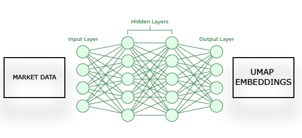
Fig 2: Visualizing our framework for estimating UMAP embeddings from given market data.

Subsequently, we will train a second model that learns to forecast future price movements in the market, given an estimation of its UMAP embeddings from our first model. Our goal is for these two statistical models, to work in a chain. The first model estimates UMAP embeddings from given market data and the second model takes the output of the first model, to forecast the future returns of the market we are trading. This framework will turn out to be considerably faster, and possibly just as effective as having implemented the UMAP algorithm from scratch. 

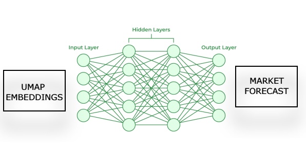
Fig 3: Visualizing our framework for generating a market forecast from our estimated UMAP embeddings

Now that we have covered our motivation and the methodology we will follow, let us get started in Python. We begin by importing the libraries we need. Readers may first need to install the UMAP library onto their machines by entering the command "pip install umap-learn", if you wish to follow along.

import pandas as pd 
import numpy as np
import matplotlib.pyplot as plt
import umap
import seaborn as sns

Otherwise, if the reader is prepared to follow along, the next step we will take is to read in the market data we generated using our MQL5 script.

HORIZON = 24
data = pd.read_csv("..\EURGBP UMAP Candlestick Recognition.csv")
data['Target'] = data['True Close'].shift(-HORIZON) - data['True Close']
data['Class'] = 0
data.loc[data['Target'] > 0,'Class'] = 1
data.dropna(inplace=True)
data

Our market data has been read in successfully, but if you look at the Time column, you will observe that we have recent market data included in our CSV file. We wish to drop the last 5 years of market data from our CSV file, so that our back test of the strategy is not tainted with leaked information our model would not have had in the past. 

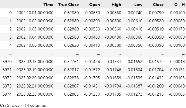
Fig 4: Our historical market data that we fetched using our MQL5 script

Let us drop off the last 5 years of market data from our CSV file. Notice that our last date in the CSV file is now the 16th of October 2019. Our back test will run from the 1st of January 2020. This gap in-between the end of our training period and the beginning of our test period is necessary to ensure that our tests are robust.

#Delete all the data that overlaps with our back test
data = data.iloc[:(-(365 * 5) + (31 * 5)),:]
data

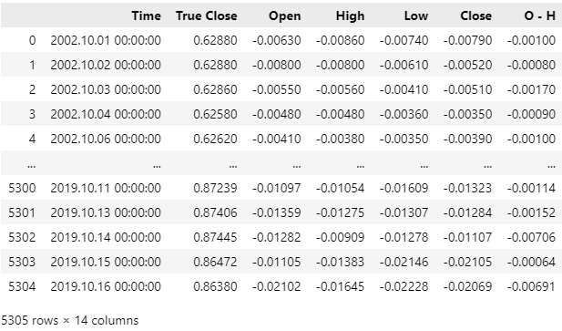
Fig 5: Be sure to drop all the data that overlaps with the period you wish to back test

Let us visualize the effects of the columns we have created for our exercise. The column "H - L" represents the difference between the Highest and Lowest price of the day. This is the effective trading range for any day. On the other hand, the column "O - C" is the net change in price for the day. By performing a scatter plot of these 2 columns, we are interested in learning if there is any relationship between the day's range and the net change for the day. Unfortunately, the relationship appears to be complicated and non-linear. This may be the type of data that UMAP can help us analyze.

sns.scatterplot(
    data=data,
    y='O - C',
    x='H - L',
    hue='Class'
)

plt.grid()
plt.title("Visualizing Our Custom Columns on EURUSD Market Data")
plt.axhline(0,color='black',linestyle='--')

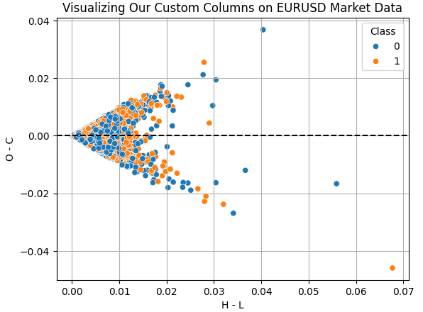
Fig 6: Visualizing the relationship between the trading range and the net change in price for the same day

Applying the UMAP transformations is rather straightforward. We first need to create a UMAP object. Afterward, we fit the UMAP object onto our data and then obtain transformed data instead. By default, our UMAP object will reduce the data down to 2 columns. We will demonstrate how to specify the desired number of columns as we progress. The 10 columns we originally fetched using our MQL5 script have been reduced down to the 2 dimensions observed in Fig 7. 

In the code example below, we are exposing certain tuning parameters of the UMAP library to the reader:

• n_neighbors: This tuning parameter instructs the algorithm how many data points should it try to ensure remain within the same neighborhood.
• metric: There are different metrics available for measuring how "close" two points are to each other, and whether they qualify as being in the same neighborhood. Changing the distance metric, will change the structure of the projected data considerably.

reducer = umap.UMAP(n_neighbors=100,metric="euclidean")

embedding = reducer.fit_transform(data.iloc[:,2:-2])
embedding = pd.DataFrame(embedding,columns=['X1','X2'])
embedding['Class'] = data['Class']

sns.scatterplot(
    data=embedding,
    x='X1',
    y='X2',
    hue='Class'
)

plt.grid()
plt.title("Visualizing the effects of UMAP on our EURUSD Market Data")

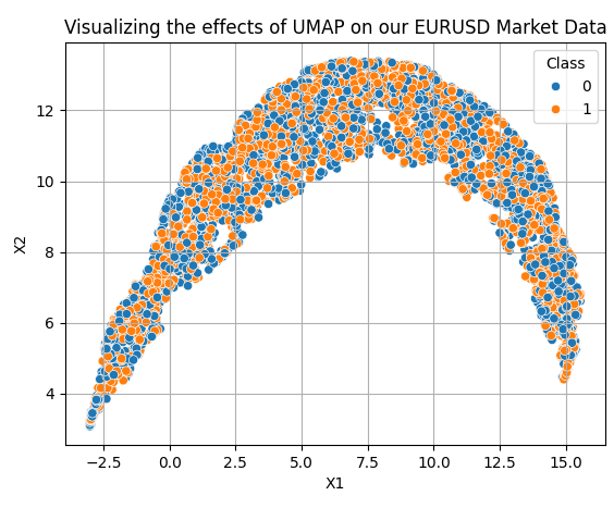
Fig 7: Visualizing our transformed data after applying the UMAP algorithm

Our new data representation is not perfect. However, it does have regions dominated by orange dots and other regions dominated by blue dots. This may make it easier for our statistical models to learn the difference between the 2 classes we are trying to distinguish. However, we only selected 2 columns arbitrarily, to give the reader a sense of how easy it is to get started. In truth, we don't know how many dimensions are required to transform the data effectively. Therefore, we will perform a line search between 1 and 9. The following function takes a parameter specifying the number of dimensions desired, and returns the corresponding transformed data to us.

def return_transformed_data(n_components):
    HORIZON = 24
    data = pd.read_csv("..\EURGBP UMAP Candlestick Recognition.csv")
    data['Target'] = data['True Close'].shift(-HORIZON) - data['True Close']
    data.dropna(inplace=True)
    data = data.iloc[:(-(365 * 5) + (31 * 5)),:]
    reducer = umap.UMAP(n_neighbors=100,metric="euclidean",n_components=n_components,n_jobs=-1)
    embedding = reducer.fit_transform(data.iloc[:,2:-1])
    cols = []
    for i in np.arange(n_components):
        s = 'X' + ' ' + str(i)
        cols.append(s)
    
    embedding = pd.DataFrame(embedding,columns=cols)
    return embedding.copy()

Now let us prepare our models.

from sklearn.ensemble import GradientBoostingRegressor
from sklearn.model_selection import TimeSeriesSplit,cross_val_score

Define the time series split object for appropriate time series cross validation.

tscv = TimeSeriesSplit(n_splits=5,gap=HORIZON)

Now let us perform the line search to figure out the optimal number of dimensions needed to represent the original data.

LEVELS = 8
res = pd.DataFrame(columns=['X'],index=np.arange(LEVELS))

for i in range(LEVELS):
    new_data = return_transformed_data(i+1)
    res.iloc[i,0] = np.mean(np.abs(cross_val_score(GradientBoostingRegressor(),new_data.iloc[:,0:],data['Target'],cv=tscv)))

Obtain the minimum index and minimum value.

res['X'] = pd.to_numeric(res['X'], errors='coerce')
min_value = min(res.iloc[:,0])
min_index = res['X'].idxmin()

Our best results were obtained when we used 3 columns to represent the original 10. The reader should understand that these are not to be thought of as the 3 best columns from the 10 we started with. Rather, the 10 columns have been transformed down to 3, 

plt.plot(res,color='black')
plt.grid()
plt.title('Finding The Optimal Number of U-MAP Components')
plt.ylabel('RMSE Validation Error')
plt.xlabel('Training Iteration')
plt.scatter(min_index,min_value,color='red')

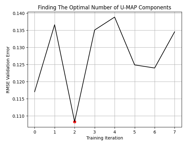
Fig 8: Our optimal number of columns were 3, from the 10 that we started with

Let us now record our error levels when using the market data in its original form.

classic_error = np.mean(np.abs(cross_val_score(GradientBoostingRegressor(),data.iloc[:,2:-2],data['Target'],cv=tscv)))

Now we shall compare the error produced by using the transformed UMAP data against the error produced when using the market data without any transformations. As we can see, the UMAP transformation has dropped our error levels to optimal regions we were not going to reach using the price data in its original form. 

results = [min(res.iloc[:,0]),classic_error]

sns.barplot(results,color='black')
plt.axhline(results[0],color='red',linestyle='--')
plt.ylabel('RMSE Validation Error')
plt.xlabel('0: UMAP Transformed Data | 1: Original OHLC Data')
plt.title("UMAP Transformations Are Helping Us Reduce Our Error Rates")

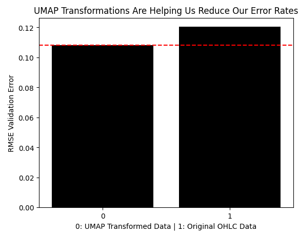
Fig 9: The UMAP transformation has reduced our error levels and is outperforming the data in its original form

Now that we have established the motivation for using UMAP transformations, we can now start building the architecture described in Fig 2 and 3. We will start by evaluating how many training iterations our neural network requires when learning how to effectively transform our original market data, into its UMAP embeddings.

from sklearn.neural_network import MLPRegressor

Fetch the required data.

new_data = return_transformed_data(3)

Perform a line search to observe the relationship between the model's error, and the number of training epochs allowed.

LEVELS = 18
NN_ERROR = pd.DataFrame(columns=['Error'],index=np.arange(LEVELS))

for i in range(LEVELS):
    model = MLPRegressor(hidden_layer_sizes=(data.iloc[:,2:-2].shape[1],10,5),max_iter=(2 ** i),solver='adam')
    NN_ERROR.iloc[i,0] =  np.mean(np.abs(cross_val_score(model,new_data,data['Target'],cv=tscv)))

Let us plot the results. Our best results were obtained when we allowed the model to perform 65 536 training iterations, or simply 2 to the power 16.

NN_ERROR['Error'] = pd.to_numeric(NN_ERROR['Error'], errors='coerce')
min_idx   = NN_ERROR.idxmin()
min_value = NN_ERROR.min()

plt.plot(NN_ERROR,color='black')
plt.grid()
plt.ylabel('5 Fold CV RMSE')
plt.xlabel('Max Iterations As Powers of 2')
plt.scatter(min_idx,min_value,color='red')
plt.title('Minimizing The Error of Our Neural Network')

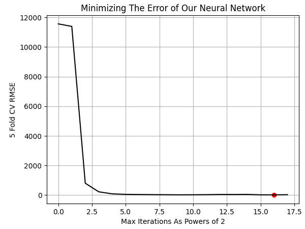
Fig 10: Visualizing the optimal number of training iterations of our model required to learn UMAP embeddings

Now we can fit both models.

#The first model will transform the given market data into its UMAP embeddings
umap_transform_model = MLPRegressor(hidden_layer_sizes=(data.iloc[:,2:-2].shape[1],10,5),max_iter=int(2 ** min_idx),solver='adam')
umap_transform_model.fit(data.iloc[:,2:-2],new_data)

#The second model will forecast the future EURGBP returns, given UMAP embeddings
forecast_model = MLPRegressor(hidden_layer_sizes=(new_data.shape[1],10,5),max_iter=int(2 ** min_idx),solver='adam')
forecast_model.fit(new_data,data['Target'])

Let us prepare to export our models to ONNX format.

import onnx
import netron
from skl2onnx import convert_sklearn
from skl2onnx.common.data_types import FloatTensorType

The model responsible for estimating our UMAP embeddings has a unique input and output shape. It takes in 10 parameters for its inputs, and returns 3 parameters for its output. We will specify this using the initial_types and final_types from the ONNX API.

umap_transform_shape = [("float_input",FloatTensorType([1,data.iloc[:,2:-2].shape[1]]))]
umap_transform_output_shape = [("float_output",FloatTensorType([new_data.shape[1],1]))]

On the other hand, the model responsible for forecasting price changes from the given UMAP embeddings, has a simple input and output shape. It takes the 3 outputs of the first model as its inputs, and only gives us 1 output.

forecast_shape = [("float_input",FloatTensorType([1,new_data.shape[1]]))]

Define the I/O shapes of the models. Notice, we must take an extra step to specify that the first model is multi-output, and then we provide the shape of our multi-output model.

umap_model_proto = convert_sklearn(umap_transform_model,initial_types=umap_transform_shape,final_types=umap_transform_output_shape,target_opset=12)
forecast_model_proto = convert_sklearn(forecast_model,initial_types=forecast_shape,target_opset=12)

Save the models.

onnx.save(umap_model_proto,"EURGBP UMAP.onnx")
onnx.save(forecast_model_proto,"EURGBP UMAP Forecast.onnx")

Getting  Started In MQL5

We can now begin writing our MQL5 code to test the profitability of UMAP regression. Recall that in Fig 5, we deleted all the data from 2020 coming towards the present. Therefore, the back test we will obtain today, gives us a fair representation of how our strategy will perform under real conditions it hasn't seen before. Let us load our ONNX models.

//+------------------------------------------------------------------+
//|                                              UMAP Regression.mq5 |
//|                                               Gamuchirai Ndawana |
//|                    https://www.mql5.com/en/users/gamuchiraindawa |
//+------------------------------------------------------------------+
#property copyright "Gamuchirai Ndawana"
#property link      "https://www.mql5.com/en/users/gamuchiraindawa"
#property version   "1.00"

//+------------------------------------------------------------------+
//| System resources                                                 |
//+------------------------------------------------------------------+
#resource "\\Files\\EURGBP UMAP.onnx" as uchar umap_onnx_buffer[];
#resource "\\Files\\EURGBP UMAP Forecast.onnx" as uchar umap_forecast_onnx_buffer[];

Additionally, we need a few global variables. Since our strategy is algorithmically driven, we will not need that many. 

//+------------------------------------------------------------------+
//| Global Variables                                                 |
//+------------------------------------------------------------------+
long umap_onnx_model,umap_forecast_onnx_model;
vectorf umap_onnx_output(3),umap_forecast_onnx_output(1);
double trade_sl;

Define handlers and buffers for our technical indicators.

//+------------------------------------------------------------------+
//| Technical indicators                                             |
//+------------------------------------------------------------------+
int ma_o_handler,ma_c_handler;
double ma_o[],ma_c[];

Load the trade library.

//+------------------------------------------------------------------+
//| Technical indicators                                             |
//+------------------------------------------------------------------+
int ma_o_handler,ma_c_handler;
double ma_o[],ma_c[];

To keep our code design human-readable, we have opted to dedicate functions to each event handler. This results in our program's body being easy to read from start to finish. If the user wishes to add more functionality, I'd advise following the same design principle and wrapping your desired utility into a method, and calling it from the body. This keeps the codebase in a state that is far easier to maintain when compared to the alternative of possibly having to parse through hundreds of lines of code, all wrapped in one event handler.

//+------------------------------------------------------------------+
//| Expert initialization function                                   |
//+------------------------------------------------------------------+
int OnInit()
  {
//---
   if(!setup())
      return(INIT_FAILED);
//---
   return(INIT_SUCCEEDED);
  }
//+------------------------------------------------------------------+
//| Expert deinitialization function                                 |
//+------------------------------------------------------------------+
void OnDeinit(const int reason)
  {
//---
   release();
  }

//+------------------------------------------------------------------+
//| Expert tick function                                             |
//+------------------------------------------------------------------+
void OnTick()
  {
//---
   update();
  }
//+------------------------------------------------------------------+

The release function cleans up for our Expert Advisor before it is completely deactivated.

//+------------------------------------------------------------------+
//| Custom functions                                                 |
//+------------------------------------------------------------------+

//+------------------------------------------------------------------+
//| Free up system memory                                            |
//+------------------------------------------------------------------+
void release(void)
  {
   IndicatorRelease(ma_c_handler);
   IndicatorRelease(ma_o_handler);
   OnnxRelease(umap_onnx_model);
   OnnxRelease(umap_forecast_onnx_model);
  }

The setup function is responsible for initializing our ONNX model and other important system variables. It returns a Boolean type that is false if something went wrong during initialization. Otherwise, the function should return to us true. The shapes of the ONNX models are paired as inputs and outputs, and their calls are also paired.

//+------------------------------------------------------------------+
//| Setup system variables                                           |
//+------------------------------------------------------------------+
bool setup(void)
  {
   umap_onnx_model = OnnxCreateFromBuffer(umap_onnx_buffer,ONNX_DATA_TYPE_FLOAT);
   umap_forecast_onnx_model = OnnxCreateFromBuffer(umap_forecast_onnx_buffer,ONNX_DATA_TYPE_FLOAT);

   ma_c_handler = iMA(_Symbol,PERIOD_CURRENT,2,0,MODE_EMA,PRICE_CLOSE);
   ma_o_handler = iMA(_Symbol,PERIOD_CURRENT,2,0,MODE_EMA,PRICE_OPEN);

   if(umap_onnx_model == INVALID_HANDLE)
     {
      Comment("Failed to create EURGBP UMAP Transformer ONNX model");
      return(false);
     }

   if(umap_forecast_onnx_model == INVALID_HANDLE)
     {
      Comment("Failed to create EURGBP UMAP Forecast ONNX model");
      return(false);
     }

   ulong umap_input_shape[]  = { 1 , 10 };
   ulong umap_forecast_input_shape[]  = { 1 , 3 };

   ulong umap_output_shape[] = { 3 , 1  };
   ulong umap_forecast_output_shape[] = { 1 , 1  };

   if(!OnnxSetInputShape(umap_onnx_model,0,umap_input_shape))
     {
      Comment("Failed to specify ONNX model input shape");
      Print("Actual shape: ",OnnxGetInputCount(umap_onnx_model));
      return(false);
     }

   if(!OnnxSetInputShape(umap_forecast_onnx_model,0,umap_forecast_input_shape))
     {
      Comment("Failed to specify EURGBP Forecast ONNX model input shape");
      Print("Actual shape: ",OnnxGetInputCount(umap_onnx_model));
      return(false);
     }

   if(!OnnxSetOutputShape(umap_onnx_model,0,umap_output_shape))
     {
      Comment("Failed to specify ONNX model output shape");
      Print("Actual shape: ",OnnxGetOutputCount(umap_onnx_model));
      return(false);
     }

   if(!OnnxSetOutputShape(umap_forecast_onnx_model,0,umap_forecast_output_shape))
     {
      Comment("Failed to specify EURGBP Forecast ONNX model output shape");
      Print("Actual shape: ",OnnxGetOutputCount(umap_onnx_model));
      return(false);
     }

   trade_sl = 2e-2;

   return(true);
  }

Our update function will help us copy indicator readings to their buffers and perform our trading routines in a periodical manner, once a day.

//+------------------------------------------------------------------+
//| Update our system variables                                      |
//+------------------------------------------------------------------+
void update(void)
  {
   static datetime time_stamp;
   datetime current_time = iTime(_Symbol,PERIOD_CURRENT,0);

   if(current_time != time_stamp)
     {
      time_stamp = current_time;

      CopyBuffer(ma_c_handler,0,0,1,ma_c);
      CopyBuffer(ma_o_handler,0,0,1,ma_o);

      if(PositionsTotal() == 0)
        {
         GetModelForecast();
         FindSetup();
        }
     }
  }

The forecast function is needed to obtain our chain of forecasts. The first forecast will be an approximation of the UMAP embeddings of the original market data. The second forecast is our trading signal, the forecasted EURGBP market return, given an approximation of its UMAP embedding.

//+------------------------------------------------------------------+
//| Get a forecast from our models                                   |
//+------------------------------------------------------------------+
void GetModelForecast(void)
  {
   vectorf model_inputs = GetUmapModelInputs();
   OnnxRun(umap_onnx_model,ONNX_DATA_TYPE_FLOAT,model_inputs,umap_onnx_output);
   OnnxRun(umap_forecast_onnx_model,ONNX_DATA_TYPE_FLOAT,umap_onnx_output,umap_forecast_onnx_output);
   Print("Model Inputs: \n",model_inputs);
   Print("Umap Transformer Forecast: \n",umap_onnx_output);
   Print("EURUSD Return UMAP Forecast: \n",umap_forecast_onnx_output);
  }

Before we can obtain a forecast from our model, we need to prepare its inputs. Recall that we must prepare the inputs of the first model, and its output will feed the second model.

//+------------------------------------------------------------------+
//| Get our model's input data                                       |
//+------------------------------------------------------------------+
vectorf GetUmapModelInputs(void)
  {
   vectorf umap_model_inputs(10);

   umap_model_inputs[0] = (float)(iOpen(_Symbol,PERIOD_CURRENT,1)  - iOpen(_Symbol,PERIOD_CURRENT,11));
   umap_model_inputs[1] = (float)(iHigh(_Symbol,PERIOD_CURRENT,1)  - iHigh(_Symbol,PERIOD_CURRENT,11));
   umap_model_inputs[2] = (float)(iLow(_Symbol,PERIOD_CURRENT,1)   - iLow(_Symbol,PERIOD_CURRENT,11));
   umap_model_inputs[3] = (float)(iClose(_Symbol,PERIOD_CURRENT,1) - iClose(_Symbol,PERIOD_CURRENT,11));
   umap_model_inputs[4] = (float)(iOpen(_Symbol,PERIOD_CURRENT,1)  - iHigh(_Symbol,PERIOD_CURRENT,1));
   umap_model_inputs[5] = (float)(iOpen(_Symbol,PERIOD_CURRENT,1)  - iLow(_Symbol,PERIOD_CURRENT,1));
   umap_model_inputs[6] = (float)(iOpen(_Symbol,PERIOD_CURRENT,1)  - iClose(_Symbol,PERIOD_CURRENT,1));
   umap_model_inputs[7] = (float)(iHigh(_Symbol,PERIOD_CURRENT,1)  - iLow(_Symbol,PERIOD_CURRENT,1));
   umap_model_inputs[8] = (float)(iHigh(_Symbol,PERIOD_CURRENT,1)  - iClose(_Symbol,PERIOD_CURRENT,1));
   umap_model_inputs[9] = (float)(iLow(_Symbol,PERIOD_CURRENT,1)   - iClose(_Symbol,PERIOD_CURRENT,1));

   return(umap_model_inputs);
  }
//+------------------------------------------------------------------+

Recall that in Fig 4 and 5 we deleted all the historical data we had that overlapped with the dates we are using in Fig 11 below. This allows us to see how our model is likely to behave when it is handling out of sample data and serves us as a true estimation of how profitable the strategy may be.

Fig 11: Our back test period for evaluating our UMAP Ensemble of models

We shall now decide the conditions under which the strategy will be tested. For the most reliable results, we will stress test the Expert Advisor under challenging conditions by giving it a random delay between its order execution and the order being filled in the back test.

Fig 12: The conditions we are simulating above, mimic real trading scenarios

In the journal of our strategy tester, we can see the inputs for our ONNX models, and the chain of UMAP models are producing valid outputs. The first model correctly reduced the 10 inputs we recorded from market data, down to 3 inputs, which were subsequently used to obtain a forecast of the market.

Fig 13: Everything appears to be working well together under the hood

Our equity curve appears to be giving us positive feedback on the performance of our system. This is encouraging because, as the reader should recall, we only approximated the UMAP algorithm and its embeddings.

Fig 14: Our strategy appears to be profitable so far

Let us take a more detailed examination of the performance of our strategy. Our system has a Sharpe Ratio of 0.42 with an expected payoff of 7.05, these are positive statistics. Our proportion of profitable trades sits at 64% while in total we placed 25 trades. 

Fig 15: A detailed analysis of our historical performance using UMAP regression

On average, each of our trades were held for 1274 hours, about 54 days. This suggests that our Expert Advisor must be catching trends in the market, for our average position time to be in the region of 54 days.

Fig 16: Visualizing the distribution of our trade durations

Upon inspection of the back test, we found that indeed the Expert Advisor was catching sustained trends in the market. In the screenshot below, the vertical white lines represent periods of 1 day, and the trades observed were placed by our UMAP Regression EA during its back test. We can observe that the first was opened in April 2020 and closed in the following month, in May. While the subsequent trade ran from the end of May until early September.

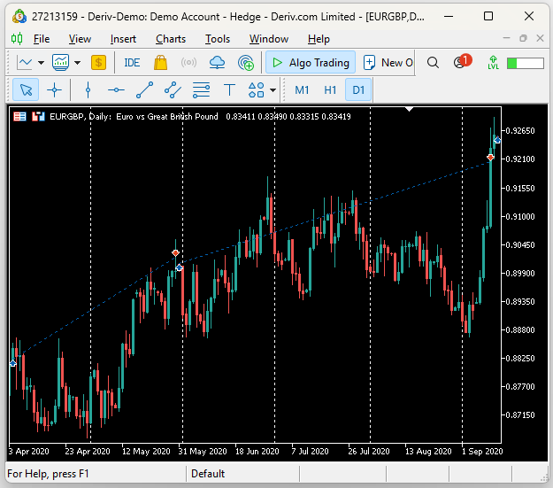
Fig 17: Visualizing the trades placed by our expert advisor

Conclusion

In this article, we have demonstrated how the reader can employ dimension reduction techniques to help their statistical model learn the dominant market features in the data they have. We showed that the UMAP algorithm can reduce our error rates when using statistical models by as much as 40% when compared to an identical model trained on the original market data without UMAP transformations. Lastly, the reader has learned a new framework that allows them to safely approximate algorithms they cannot implement natively. This should leave you with a competitive edge in any market you decide to trade.

File Name	Description
EURGBP UMAP Forecast.onnx	ONNX file that takes our approximated UMAP embeddings as its input, to forecast the future EURGBP return.
EURGBP UMAP.onnx	ONNX file responsible for taking our market data as its input, and approximating the correct UMAP embeddings.
UMAP Candlestick Recognition.ipynb	The Jupyter Notebook we used to analyze our MetaTraer 5 market data and build our ONNX files.
UMAP Candlestick Recognition.mq5	The MQL5 script file we built to fetch our detailed market data.
UMAP Regression.mq5	The expert advisor we built to trade the EURGBP using our two model architecture.