From Basic to Intermediate: Queues, Lists, and Trees (I)

Introduction

In our previous article, "From Basic to Intermediate: Like Bubbles", we showed how to implement a very simple sorting mechanism. Although this may not be very efficient in terms of execution time, in many cases this approach is suitable for a wide range of situations where the goal is to sort a set of data and, by doing so, simplify the task of interpreting it and performing simple searches within it.

The mechanism described in the previous article does not always operate on its own. Most often, sorting and searching systems are linked to other types of mechanisms. In this article, we will examine one of these mechanisms.

Indeed, although we are still focusing on basic topics, some people might find the material covered here to be more advanced. However, all of this is related to the fundamentals that every professional programmer should know.

All right, to get off on the right foot, let's move on to a new topic. Please keep in mind that if you have trouble understanding the information presented here, or if the discussion involves topics not covered in this article, you should refer to previous articles. There you will find all the information you need to understand this article.

Queues, Lists, and Trees (I)

There is a kind of material that many beginners end up neglecting because they consider it unnecessary, even though it is actually something they should master and understand very well. This material, which beginners often underestimate, is aimed precisely at ensuring proper data analysis and structuring.

Attention, dear reader! There is no point in learning how to create an Expert Advisor or even a simple indicator if you don't know how to properly analyze all the data the application generates. Now pause for a moment and think about it. If you understand how to analyze and categorize the data the application receives, you can streamline its operation, and as a result, it will run faster.

There is currently a lot of excitement surrounding machine learning and related topics. However, even artificial intelligence systems are nothing more than simple classifiers and statistical data analysis systems. Under no circumstances do these systems possess true intelligence capable of surpassing human creativity and the ability to understand a particular subject.

In other words, ultimately, although artificial intelligence or machine learning—which many consider the pinnacle of technology—may seem amazing, they are nothing more than algorithms capable of applying a number of fundamentals that every good programmer should master. Understanding how—and, more importantly, why—you should use this particular implementation model rather than another can be crucial. You'll only be able to master this art over time, through good practice and experience. The purpose of these articles is not to tell you when to use a particular implementation model, but rather to introduce these models and show how they can be used with MQL5 to generate results in MetaTrader 5.

So, there is a certain logical sequence—if you can call it that—in the presentation of the material we will be discussing here. And since I want to be as clear as possible—and some beginners might not grasp the importance of this material—let's start with the simplest implementation: queues.

In principle, a queue can resemble an array. Despite this similarity, a queue can take various forms, some of which differ greatly from one another. Thus, these forms may serve entirely different purposes depending on the specific circumstances and how they are implemented. Precisely because they are so similar to data arrays, many beginners often confuse them with arrays—and for good reason. However, queues are not necessarily arrays, since their purpose and the way they are processed differ significantly from arrays themselves.

Since queues can have very distinct and, at the same time, quite interesting characteristics—and can even have very exotic implementations depending on the features offered by the language—we’ll start with something very simple. The fact is that the concept and functioning of classes have not yet been explained. Nevertheless, enough material has already been presented for us to be able to implement various structures without much difficulty. Therefore, we can write—or, more precisely, implement—the code shown below.

01. //+------------------------------------------------------------------+
02. #property copyright "Daniel Jose"
03. //+------------------------------------------------------------------+
04. template <typename T> struct stFIFO
05. {
06.     private:
07. //+----------------+
08.         T   value[];
09. //+----------------+
10.     public:
11. //+----------------+
12.     T Restore(void)
13.     {
14.         T local = NULL;
15. 
16.         if (value.Size() > 0)
17.         {
18.             local = value[0];
19.             ArrayRemove(value, 0, 1);
20.         };
21.         return local;
22.     };
23. //+----------------+
24.     void Stock(T arg)
25.     {
26.         T local[1];
27.         local[0] = arg;
28.         ArrayInsert(value, local, value.Size());
29.     }
30. //+----------------+
31. };
32. //+------------------------------------------------------------------+
33. void OnStart(void)
34. {
35.     stFIFO <char> fifo;
36. 
37.     fifo.Stock(10);
38.     fifo.Stock(84);
39.     fifo.Stock(-6);
40. 
41.     Print(fifo.Restore());
42.     Print(fifo.Restore());
43.     Print(fifo.Restore());
44.     Print(fifo.Restore());
45. }
46. //+------------------------------------------------------------------+

Code 01

So, this is our first step toward a broader understanding of these data structures, known in programming as queues, lists, and trees. Now, dear reader, I'd like you to take a closer look at some details in this code. Please note that on line 08, we declare a dynamic array, and this array can hold values of any type, as you can see just by looking at the declaration on line 08.

This array should not be viewed in the same way as the ones we have seen so far. The reason is in the function on line 12 and the procedure on line 24. These procedures and functions can have any name. What really matters is how they work. So please pay close attention to the explanation that follows. This is because, depending on the functions and procedures involved, and the structure being implemented can change very quickly. This could lead to a change in the type of queue or even trigger radical changes, to the point where we implement a list or even a tree instead of a queue.

This is the easiest part. If you look at the code for the Restore function on line 12, you will see that when the array declared on line 08 contains data, we always take the data from index 0 of that array so that we can later return it to the caller. The most important thing here is what line 19 will actually do. Its purpose is to remove the element at index 0. "But wait a minute. I don't get it. If we always return the contents of index 0, then when we remove that very index, we’ll end up creating a certain inconsistency in the code. Because on the next call, the zero index will not contain any data."

Well, dear reader, in reality, things won't quite turn out that way. As I mentioned earlier, many beginners confuse these concepts precisely because they only skim the code without understanding what’s going on underneath. But I guarantee that you will soon understand everything better. Just listen carefully to what I will explain.

So now we know that the function on line 12 will always return the contents at index 0 of the array. What about the procedure on line 24? What does it do? All right, in this case, this procedure stores the data passed to it in an array. However, this same data will always be stored at the end of the array. "Hmm, I don't get it. Could you explain that in a little more detail?"

Yes, dear reader. You already know that an array can have various indices, ranging from zero to any value. When the first value is passed to the Stock procedure on line 24, it is stored at index 0. So far, so good, because when we use the Restore function, we will read exactly the contents at index 0. This is exactly where many beginner programmers get confused. The next data item sent to Stock will be stored at index 1. This happens because data already exists at index 0. The next element will be stored at index 2 for the same reason: there is already data at index 1. And so on.

However, in any of these situations, the Restore function will always continue to read the contents at index 0. But this is where the explanation gets interesting. When you use the Restore function, the remaining elements shift down by one position. That's how we create a processing queue. To see this in action, let's take a look at the list of commands in the OnStart procedure, starting at line 33. When lines 37 through 39 are executed, a queue will be created in exactly the same order in which we declared the values. Conversely, when we execute lines 41 through 44, we will read what was inserted into the queue. It might seem a little strange, but it works. The execution result is shown in the following image.

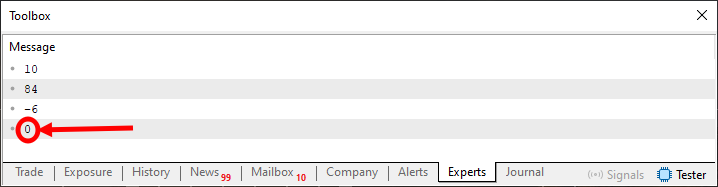
Image 01

Please note that a different element is highlighted in Image 01. The Restore function returns it because there are no more elements in the queue. This happens because, in line 14, we declare what value will be returned when there is no data in the array declared in line 08.

It is clear that even though we always access index 0 in the Restore function, we can still see the data that was inserted into the queue. This type of queue has a specific name: FIFO — which stands for first in, first out. Try running a few tests to get a better understanding of this. For example, add several values to the queue, read some of them, and then add more values. Try to understand how the read and write operations work.

This type of queue is very useful in various situations where we need to analyze data in a specific order and must not lose track of that order. Therefore, before moving on to the next option, it is a good idea to practice and understand how this first code snippet works.

In the code below, which we'll look at in a moment, we will create a different type of queue with a completely different purpose than the one we discussed earlier. But before you try to understand what will happen in the next code snippet, I strongly recommend that you, dear reader, take some time to truly understand what was shown in Code 01 and how it works. This will help avoid confusion regarding what we will see in the following code.

01. //+------------------------------------------------------------------+
02. #property copyright "Daniel Jose"
03. //+------------------------------------------------------------------+
04. template <typename T> struct stQueue
05. {
06.     private:
07. //+----------------+
08.         T       value[];
09.         uint    c_Pos,
10.                 c_Max;
11. //+----------------+
12.     public:
13. //+----------------+
14.     void Init(uint arg)
15.     {
16.         ArrayResize(value, arg + 1);
17.         c_Pos = c_Max = 0;
18.     }
19. //+----------------+
20.     bool GetInfo(T &arg)
21.     {
22.         if (c_Pos == c_Max)
23.             return false;
24.         c_Pos = (c_Pos < value.Size() - 1 ? c_Pos + 1 : 0);
25.         arg = value[c_Pos];
26. 
27.         return true;
28.     }
29. //+----------------+
30.     void Stock(const T arg)
31.     {
32.         c_Max = (c_Max < value.Size() - 1 ? c_Max + 1 : 0);
33.         c_Pos = (c_Pos == c_Max ? (c_Pos < value.Size() - 1 ? c_Pos + 1 : 0) : c_Pos);
34.         value[c_Max] = arg;
35.     }
36. //+----------------+
37. };
38. //+------------------------------------------------------------------+
39. void OnStart(void)
40. {
41.     stQueue <char> Queue;
42. 
43.     Queue.Init(5);
44. 
45.     Queue.Stock(10);
46.     Queue.Stock(84);
47.     Queue.Stock(-6);
48.     Queue.Stock(15);
49.     Queue.Stock(-35);
50.     Queue.Stock(40);
51.     Queue.Stock(-35);
52. 
53.     for (char info; Queue.GetInfo(info);)
54.         Print(info);
55. }
56. //+------------------------------------------------------------------+

Code 02

In Code 02, we implement another type of queue, known among programmers as a circular queue. Although this type of implementation is simpler when using classes, there is nothing stopping us from implementing it using the resources already described in previous articles. When we implement this using classes, you will see that everything becomes much simpler—both when creating it and when using the implementation presented here. But that is a topic for another time. Let's focus on what we have right now.

And now, dear reader, please pay even closer attention. If Code 01 seemed a little confusing and complicated to you, then Code 02 will confuse you even more, because here we are doing something that might seem like pure madness to many people. Although, in practice, this can be very useful in many situations. Please note that part of the structure declared in line 04 of Code 02 is very similar to what was done in Code 01. It even contains very similar fragments. However, the version implemented here differs significantly from what was done in Code 01. And not only that. In this case, when using Code 02—unlike Code 01—some data may be lost.

"But wait a minute. How is it even possible for data to be lost? Doesn't that create a problem for the code?" No, actually it doesn't, dear reader. There are situations where this is to be expected—or, in other words, we can lose data without worrying that it will affect the final result. This might seem a little strange to many of you. But let's take a look at the moving averages used on the chart. Moving averages, in a sense, function as a queue of values, where the oldest ones are discarded. For example, a 20-period moving average stores 20 values: the first is the most recent, and the last one is discarded as soon as a newer value is added to the queue.

Now pay attention, because this is important. Since we have a fixed range of values and they are replaced by newer ones, we should refer to this type of structure as a queue rather than a list. Lists of values serve a different purpose; queues, on the other hand, have a very simple and practical purpose. These two terms are often confused. However, to avoid any confusion regarding interpretation, we refer to the structure shown here as a queue. Although at first glance this may seem like just a list of values.

All right, now note that in the case of a circular queue, we need a way to limit the range or number of values in the queue. This is done using the procedure described on line 14. Here, we specify the number of values the queue will contain; this number can be any value greater than zero. Thus, on line 16, we allocate enough memory for the dynamic array created on line 08. However, since we are initializing our circular queue, we also need to initialize two additional values. This is done on line 17. Thus, the queue has been created and is ready to receive data or have data read from it.

This is the point at which many people, encountering this approach for the first time, often feel quite confused. Since we need to read elements from the queue, we implemented the function on line 20. This function returns any element from the queue. Which element? Well, that depends on the circumstances, dear reader. To understand the reason behind my answer, note that a check is performed on line 22. If the value of `c_Pos`, which indicates the current read position, is equal to the value of `c_Max`, which indicates the current write position, then there are no elements to return. Therefore, the check on line 22 may return `false` in some cases.

If this does not happen, it means that there is some value available to read. In this situation, we use line 24 to calculate a new read position within the queue. Why do we need this calculation? Wouldn't it be easier to increment the value of the `c_Pos` counter? No, not really, dear reader. This is because we are working with a circular queue: if its size is smaller than the full range of values of the `uint` type, the index must wrap around to the beginning, as is done on line 24. As a result, the `c_Pos` counter will point back to index 01 of the array as soon as it reaches the upper bound of the queue. That is how a circular queue is created. The rest of the code is simple.

So, let's move on to the procedure on line 30, since it is responsible for a very interesting and, at the same time, highly intriguing operation. Note the following: on line 32, we find logic very similar to that on line 24, with the only difference that the variable that is subject to adjustment, changes. But the goal remains the same: to return to the beginning of the array as soon as the maximum number of elements allocated on line 16 is reached.

"Wait a second—now things are really getting complicated. I say this because I notice that the same value, `c_Max`, is used on line 34 to specify the index at which the value we provide will be stored. However, you state that line 32 will periodically return to the zero index. After all, if we can store 20 elements and we store 21 (that is, one more than the limit defined on line 16), will we be able to read only one element?” No, dear reader. We will still be able to read the 20 items that have already been saved. However, the first element stored in the queue will be replaced by this new element—the 21st element. "What a convoluted explanation. I don't understand how we'll be able to do this." Don't worry, you will understand everything soon. However, to ensure that this read capability is preserved throughout the entire circular queue, you need to implement line 33. This line advances the queue without having to shift the array elements.

Please note: when c_Max equals c_Pos, this means that the queue is full. Otherwise, these values will never be equal. Since the queue is already full, we forcibly move c_Pos to the next position. However, to ensure that `c_Pos` points to the next valid position in the queue, we use a second ternary operator, thereby ensuring that the bounds of the circular queue are respected. Therefore, this second ternary operator is exactly the same as the operator on line 24. Since I know that most of you are beginners and may have some trouble understanding Code 02, you will find a slightly modified version of the code in the attachment. The code is shown below:

01. //+------------------------------------------------------------------+
02. #property copyright "Daniel Jose"
03. //+------------------------------------------------------------------+
04. template <typename T> struct stQueue
05. {
06.     #define macro_AdjustLimit(A) (A < value.Size() - 1 ? A + 1 : 0)
07. //+----------------+
08.     private:
09. //+----------------+
10.         T       value[];
11.         uint    c_Pos,
12.                 c_Max;
13. //+----------------+
14.     public:
15. //+----------------+
16.     void Init(uint arg)
17.     {
18.         ArrayResize(value, arg + 1);
19.         c_Pos = c_Max = 0;
20.     }
21. //+----------------+
22.     bool GetInfo(T &arg)
23.     {
24.         if (c_Pos == c_Max)
25.             return false;
26.         c_Pos = macro_AdjustLimit(c_Pos);
27.         arg = value[c_Pos];
28. 
29.         return true;
30.     }
31. //+----------------+
32.     void Stock(const T arg)
33.     {
34.         c_Max = macro_AdjustLimit(c_Max);
35.         c_Pos = (c_Pos == c_Max ? macro_AdjustLimit(c_Pos) : c_Pos);
36.         value[c_Max] = arg;
37.     }
38. //+----------------+
39.     #undef macro_AdjustLimit
40. //+----------------+
41. };
42. //+------------------------------------------------------------------+
43. void OnStart(void)
44. {
45.     stQueue <char> Queue;
46. 
47.     Queue.Init(5);
48. 
49.     Queue.Stock(10);
50.     Queue.Stock(84);
51.     Queue.Stock(-6);
52.     Queue.Stock(15);
53.     Queue.Stock(-35);
54.     Queue.Stock(40);
55.     Queue.Stock(-35);
56. 
57.     for (char info; Queue.GetInfo(info);)
58.         Print(info);
59. }
60. //+------------------------------------------------------------------+

Code 03

Code 03 does the same thing as Code 02. The only difference is in the definition of the macro on line 06 in this Code 03. However, this makes it somewhat easier to understand line 33 of Code 02. This is because line 35 of Code 03 is much easier to read. Although this is the same line as line 33 in Code 02, it is easier to read.

However, we are more interested in how this structure works and how it creates and maintains what is known as a circular queue. To test this structure, which creates a circular queue, we use the contents of the OnStart procedure.

Now let's focus on Code 03. This way, we will be able to follow the specified lines. First, we define the queue itself. The definition is given on line 45. Next, we determine how many elements the queue will contain. In this case, it is specified on line 47. Note that in this case, we specify that the number of elements will be a MAXIMUM of five.

Now comes the most interesting part—using a circular queue. To do this, we use lines 49 through 55. Please note the following: we have a queue that can contain up to five elements. However, we ask to add seven elements to this queue. Question: What will happen here? Answer: Older elements will be overwritten as the queue advances. How can we be sure of that? So, to do this, we use line 57, where a loop appears that might seem intriguing at first glance. However, in another article, I clearly explained how we can work with the `for` statement to create loops for some very interesting purposes. This is one such case. Note that the loop itself creates the necessary conditions for running and terminating. We are interested in the execution of line 58. This line lets us see which elements have been removed and which remain in the queue.

So, when we run Code 03 or Code 02, we get the result shown in the following image:

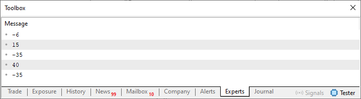
Image 02

That's all, dear reader. I want you to pause for a moment and think about the result shown in Image 02. And compare this with the contents of Code 03, between lines 49 and 55. Do you understand what's going on here? Can you identify any connection between what was shown in Code 01, where we implemented a FIFO queue (first in, first out), and this circular queue, which is implemented in Code 03? Yes? No? Maybe. You probably do not see the connection, but there is a connection between what was explained at the beginning of this article and what we see here. The point is this: the first element in the queue is always retrieved first. Similarly, the last element in the queue is the last element to be displayed. Unlike previous methods, here we limit the number of elements that can be in the queue. This limit is defined on line 47 of Code 03.

This is where the confusion arises—and it is something many people don't understand. When we start programming, we waste a lot of time trying to create or implement something. However, it is quite likely that an implementation of what we are trying to do already exists somewhere. Now consider the following: suppose you are creating an Expert Advisor to analyze a moving average with a period of X. "Why store more than X price values? That makes no sense." Similarly, there is no point in modifying price data just to keep an array of X price values up to date. All you need to do is create or implement a data structure such as a circular queue. The implementation itself will ensure that prices always stay up to date, with virtually no shift operations, since the index counters we use will perform this shift for us. As a result, the executable code runs much faster and is easier to maintain.

Final Thoughts

In this article, we began exploring one of the least-known topics among beginner programmers. People often desperately want to learn how to program, but do not try to understand the fundamental concepts. In my opinion, a proper understanding of these concepts is far more important and necessary than endlessly writing code. This is because a proper understanding of certain concepts can help us write code that is much safer, faster, and easier to maintain.

So, dear reader, take your time studying and putting into practice what you have learned from this article. It took me quite a while to grasp these fundamentals, which I am trying to convey to you. When I was studying this topic, no one paid much attention to it. Everyone demanded only results from us, regardless of how we achieved them. But here, I am showing you this path. You will need to learn how to find your way through it. This way, your learning process will be as smooth and consistent as possible. Take your time. Study and put into practice what we have learned in this article. In the next article, we will continue our discussion of queues, lists, and trees.

File	Description
Code 01	Simple queue
Code 02	Simple queue