
Integrating MQL5 with data processing packages (Part 3): Enhanced Data Visualization

Introduction
Traders in the financial markets often face the challenge of making sense of vast amounts of data, from price fluctuations and trading volumes to technical indicators and economic news. With the speed and complexity of modern markets, it becomes overwhelming to interpret these data streams effectively using traditional methods. Charts alone may not provide enough insight, leading to missed opportunities or poorly timed decisions. The need to quickly identify trends, reversals, and potential risks adds to the difficulty. For traders looking to make informed, data-driven decisions, the inability to distill key insights from data is a critical problem that can result in lost profits or heightened risks.
Enhanced data visualization addresses this challenge by transforming raw financial data into more intuitive and interactive visual representations. Tools like dynamic candlestick charts, overlays of technical indicators, and heat-maps of returns provide traders with a deeper, more actionable understanding of market conditions. By integrating visual elements that highlight trends, correlations, and anomalies, traders can quickly spot opportunities and make better-informed decisions. This enhanced approach helps reduce the complexity of interpreting data, enabling traders to act more confidently and efficiently in the fast-moving financial markets.
Gather Historical Data
from datetime import datetime
import MetaTrader5 as mt5
import pandas as pd
import pytz

# Display data on the MetaTrader 5 package
print("MetaTrader5 package author: ", mt5.__author__)
print("MetaTrader5 package version: ", mt5.__version__)

# Configure pandas display options
pd.set_option('display.max_columns', 500)
pd.set_option('display.width', 1500)

# Establish connection to MetaTrader 5 terminal
if not mt5.initialize():
    print("initialize() failed, error code =", mt5.last_error())
    quit()

# Set time zone to UTC
timezone = pytz.timezone("Etc/UTC")
# Create 'datetime' objects in UTC time zone to avoid the implementation of a local time zone offset
utc_from = datetime(2024, 1, 2, tzinfo=timezone)
utc_to = datetime.now(timezone)  # Set to the current date and time

# Get bars from XAUUSD H1 (hourly timeframe) within the specified interval
rates = mt5.copy_rates_range("XAUUSD", mt5.TIMEFRAME_H1, utc_from, utc_to)

# Shut down connection to the MetaTrader 5 terminal
mt5.shutdown()

# Check if data was retrieved
if rates is None or len(rates) == 0:
    print("No data retrieved. Please check the symbol or date range.")
else:
    # Display each element of obtained data in a new line (for the first 10 entries)
    print("Display obtained data 'as is'")
    for rate in rates[:10]:
        print(rate)

    # Create DataFrame out of the obtained data
    rates_frame = pd.DataFrame(rates)
    # Convert time in seconds into the 'datetime' format
    rates_frame['time'] = pd.to_datetime(rates_frame['time'], unit='s')

    # Save the data to a CSV file
    filename = "XAUUSD_H1_2nd.csv"
    rates_frame.to_csv(filename, index=False)
    print(f"\nData saved to file: {filename}")
To retrieve historical data, we first establish a connection to the MetaTrader 5 terminal using the `mt5.initialize()` function. This is essential because the Python package communicates directly with the running MetaTrader 5 platform. We configure the code to set the desired time range for data extraction by specifying the start and end dates. The `datetime` objects are created in the UTC time zone to ensure consistency across different time zones. The script then uses the `mt5.copy-rates-range()` function to request historical hourly data for the XAUUSD symbol, starting from January 2, 2024, up to the current date and time.
After obtaining the historical data, we safely disconnect from the MetaTrader 5 terminal using `mt5.shutdown()` to avoid any further unnecessary connections. The retrieved data is initially displayed in its raw format to confirm successful data extraction. We convert this data into a pandas DataFrame for easier manipulation and analysis. Additionally, the code converts the Unix timestamps into a readable datetime format, ensuring the data is well-structured and ready for further processing or analysis. This approach allows traders to analyze historical market movements and make informed trading decisions based on past performance.
filename = "XAUUSD_H1_2nd.csv"
rates_frame.to_csv(filename, index=False)
print(f"\nData saved to file: {filename}")
Since my Operating System is Linux I have to save the received data into a file. But for those who are on Windows, you can simply retrieve the data with the following script:
from datetime import datetime
import MetaTrader5 as mt5
import pandas as pd
import pytz

# Display data on the MetaTrader 5 package
print("MetaTrader5 package author: ", mt5.__author__)
print("MetaTrader5 package version: ", mt5.__version__)

# Configure pandas display options
pd.set_option('display.max_columns', 500)
pd.set_option('display.width', 1500)

# Establish connection to MetaTrader 5 terminal
if not mt5.initialize():
    print("initialize() failed, error code =", mt5.last_error())
    quit()

# Set time zone to UTC
timezone = pytz.timezone("Etc/UTC")
# Create 'datetime' objects in UTC time zone to avoid the implementation of a local time zone offset
utc_from = datetime(2024, 1, 2, tzinfo=timezone)
utc_to = datetime.now(timezone)  # Set to the current date and time

# Get bars from XAUUSD H1 (hourly timeframe) within the specified interval
rates = mt5.copy_rates_range("XAUUSD", mt5.TIMEFRAME_H1, utc_from, utc_to)

# Shut down connection to the MetaTrader 5 terminal
mt5.shutdown()

# Check if data was retrieved
if rates is None or len(rates) == 0:
    print("No data retrieved. Please check the symbol or date range.")
else:
    # Display each element of obtained data in a new line (for the first 10 entries)
    print("Display obtained data 'as is'")
    for rate in rates[:10]:
        print(rate)

    # Create DataFrame out of the obtained data
    rates_frame = pd.DataFrame(rates)
    # Convert time in seconds into the 'datetime' format
    rates_frame['time'] = pd.to_datetime(rates_frame['time'], unit='s')

    # Display data directly
    print("\nDisplay dataframe with data")
    print(rates_frame.head(10))
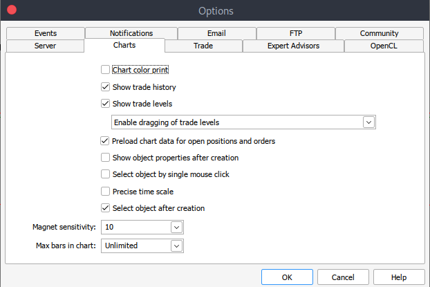
And if for some reason, you can't get historical data, you can retrieve it manually on your MetTrader5 platform with the following steps. Launch your MetaTrader platform and at the top of your MetaTrader 5 pane/panel navigate to > Tools and then > Options and you will land to the Charts options. You will then have to select the number of Bars in the chart you want to download. It's best to choose the option of unlimited bars since we'll be working with date, and we wouldn't know how many bars are there in a given period of time.
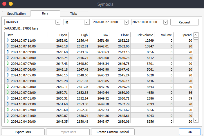
After that, you will now have to download the actual data. To do that, you will have to navigate to > View and then to > Symbols, and you will land on the Specifications tab. Simply navigate to > Bars or Ticks depending on what kind of data want to download. Proceed and enter the start and end date period of the historical data you would like to download, after that, click on the request button to download the data and save it in the .csv format.
MetaTrader 5 Data Visualization on Jupyter Lab
To load your MetaTrader 5 historical data into Jupyter Lab, you first need to locate the folder where the data was downloaded. Once in Jupyter Lab, navigate to that folder to access the files. The next step is to load the data and review the column names. Inspecting the column names is important to ensure that you manage the data correctly and prevent errors that could occur from using incorrect column names.
Python code:
import pandas as pd

# assign variable to the historical data
file_path = '/home/int_junkie/Documents/ML/predi/XAUUSD.m_H1_2nd.csv'

data = pd.read_csv(file_path, delimiter='\t')

# Display the first few rows and column names
print(data.head())
print(data.columns)
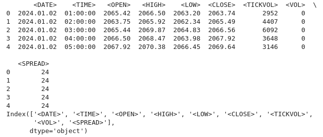
Our historical data starts from January 2, 2024, until current data.
Python code:
# Convert the <DATE> and <TIME> columns into a single datetime column
data['<DATETIME>'] = pd.to_datetime(data['<DATE>'] + ' ' + data['<TIME>'], format='%Y.%m.%d %H:%M:%S')

# Drop the original <DATE> and <TIME> columns
data = data.drop(columns=['<DATE>', '<TIME>'])

# Convert numeric columns from strings to appropriate float types
numeric_columns = ['<OPEN>', '<HIGH>', '<LOW>', '<CLOSE>', '<TICKVOL>', '<VOL>', '<SPREAD>']
data[numeric_columns] = data[numeric_columns].apply(pd.to_numeric)

# Set datetime as index for easier plotting
data.set_index('<DATETIME>', inplace=True)

# Let's plot the close price and tick volume to visualize the trend
import matplotlib.pyplot as plt

# Plot closing price and tick volume
fig, ax1 = plt.subplots(figsize=(12, 6))

# Close price on primary y-axis
ax1.set_xlabel('Date')
ax1.set_ylabel('Close Price', color='tab:blue')
ax1.plot(data.index, data['<CLOSE>'], color='tab:blue', label='Close Price')
ax1.tick_params(axis='y', labelcolor='tab:blue')

# Tick volume on secondary y-axis
ax2 = ax1.twinx()
ax2.set_ylabel('Tick Volume', color='tab:green')
ax2.plot(data.index, data['<TICKVOL>'], color='tab:green', label='Tick Volume')
ax2.tick_params(axis='y', labelcolor='tab:green')

# Show the plot
plt.title('Close Price and Tick Volume Over Time')
fig.tight_layout()
plt.show()

The plot above shows two key metrics over time:
- Close Price (in blue): This represents the closing price for each hour on the chart. We can observe fluctuations over time, indicating periods of both upward and downward trends in the price of gold (XAU/USD).
- Tick Volume (in green): This indicates the number of price changes within each hour. Spikes in tick volume often correspond to increased market activity or volatility. For example, periods of high volume may coincide with significant price movements, which could signal important events or shifts in market sentiment.
Now let's dip deeper into our data:
1. Trend Analysis.
# Calculating moving averages: 50-period and 200-period for trend analysis
data['MA50'] = data['<CLOSE>'].rolling(window=50).mean()
data['MA200'] = data['<CLOSE>'].rolling(window=200).mean()

# Plot close price along with the moving averages
plt.figure(figsize=(12, 6))

# Plot close price
plt.plot(data.index, data['<CLOSE>'], label='Close Price', color='blue')

# Plot moving averages
plt.plot(data.index, data['MA50'], label='50-Period Moving Average', color='orange')
plt.plot(data.index, data['MA200'], label='200-Period Moving Average', color='red')

plt.title('Close Price with 50 & 200 Period Moving Averages')
plt.xlabel('Date')
plt.ylabel('Price')
plt.legend(loc='best')
plt.grid(True)
plt.show()
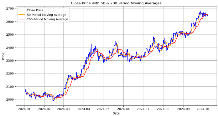
The plot shows the closing price along with the 50-period and 200-period moving averages:
- Close Price (blue line): This represents the actual price at the end of each time period.
- 50-period Moving Average (orange line): A shorter-term moving average that smooths out price data over 50 periods. When the close price crosses above this line, it can signal a potential upward trend, and when it crosses below, it may indicate a downward trend.
- 200-period Moving Average (red line): A longer-term moving average, which provides insights into the overall trend. It tends to react more slowly to price changes, so crossovers with the 50-period moving average can signal significant long-term trend reversals.
The key point we are looking for is the golden cross, when the 50-period moving average crosses above the 200-period moving average, it can signal a potential strong bullish trend. The last one being the death cross, which is when the 50-period moving average crosses below the 200-period moving average, it may signal a potential bearish trend.
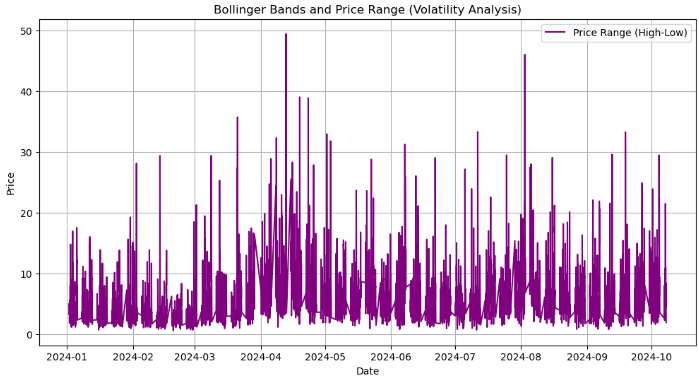
Next, we analyze the volatility by calculating the price range (difference between the high and low) and visualize it.
2. Volatility Analysis.
# Calculate the price range (High - Low)
data['Price_Range'] = data['<HIGH>'] - data['<LOW>']

# Calculate Bollinger Bands
# Use a 20-period moving average and 2 standard deviations
data['MA20'] = data['<CLOSE>'].rolling(window=20).mean()
data['BB_upper'] = data['MA20'] + 2 * data['<CLOSE>'].rolling(window=20).std()
data['BB_lower'] = data['MA20'] - 2 * data['<CLOSE>'].rolling(window=20).std()

# Plot the price range and Bollinger Bands along with the close price
plt.figure(figsize=(12, 8))

# Plot the close price
plt.plot(data.index, data['<CLOSE>'], label='Close Price', color='blue')

# Plot Bollinger Bands
plt.plot(data.index, data['BB_upper'], label='Upper Bollinger Band', color='red', linestyle='--')
plt.plot(data.index, data['BB_lower'], label='Lower Bollinger Band', color='green', linestyle='--')

# Fill the area between Bollinger Bands for better visualization
plt.fill_between(data.index, data['BB_upper'], data['BB_lower'], color='gray', alpha=0.3)

# Plot the price range on a separate axis
plt.figure(figsize=(12, 6))
plt.plot(data.index, data['Price_Range'], label='Price Range (High-Low)', color='purple')

plt.title('Bollinger Bands and Price Range (Volatility Analysis)')
plt.xlabel('Date')
plt.ylabel('Price')
plt.legend(loc='best')
plt.grid(True)
plt.show()
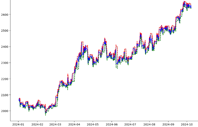
From the output above, we have done the following:
- Price Range Calculation: We calculate the price range for each time period by subtracting the lowest price (`<LOW>`) from the highest price ('<High>`). This gives the extent of price movement during each hour, helping to measure the volatility for that period.
- `data['Price-Range'] = data['<HIGH>'] - data['<LOW>'] : The resulting `Price-Range` column shows how much the price fluctuated within each hour.
- Bollinger Bands Calculation: The Bollinger bands indicator is calculated, in insights into price volatility. `MA-20` Is the 20-period moving average of the closing prices. It serves as the middle line of the Bollinger Bands. `BB-upper` and `BB-lower` represent the upper and lower bands, respectively. They are calculated as two standard deviations above and below the 20-period moving average. When prices move towards the upper band, it indicates that the market might be overbought; similarly, movements towards the lower band suggest the market might be oversold.
- Visualization of Price and Bollinger Bands: Close Price (blue line), represents the actual close price for each time period. Upper Bollinger Bands (red dashed line) and Lower Bollinger Bands (green dashed line), these lines show the volatility bands that form the Bollinger Bands around the moving average. Shaded area, the area between the upper and lower Bollinger Bands is shaded gray, visually representing the volatility range within which the price is expected to move.
- Separate Price Range Plot: The second plot displays the Price Range as a separate purple line, showing how the volatility fluctuates over time. Larger spikes in this plot indicate periods of increased volatility.
import pandas as pd
import talib
from stable_baselines3 import DQN
from stable_baselines3.common.env_checker import check_env

# Verify the environment
check_env(env)

# Initialize and train the DQN model
model = DQN('MlpPolicy', env, verbose=1)
model.learn(total_timesteps=10000)

# Save the trained model
model.save("trading_dqn_model")

# Load and preprocess the data as before
data = pd.read_csv('XAUUSD_H1_Data-V.csv', delimiter='\t')
data['<DATETIME>'] = pd.to_datetime(data['<DATE>'] + ' ' + data['<TIME>'], format='%Y.%m.%d %H:%M:%S')
data = data.drop(columns=['<DATE>', '<TIME>'])
numeric_columns = ['<OPEN>', '<HIGH>', '<LOW>', '<CLOSE>', '<TICKVOL>', '<VOL>', '<SPREAD>']
data[numeric_columns] = data[numeric_columns].apply(pd.to_numeric)
data.set_index('<DATETIME>', inplace=True)

# Calculate Bollinger Bands (20-period moving average with 2 standard deviations)
data['MA20'] = data['<CLOSE>'].rolling(window=20).mean()
data['BB_upper'] = data['MA20'] + 2 * data['<CLOSE>'].rolling(window=20).std()
data['BB_lower'] = data['MA20'] - 2 * data['<CLOSE>'].rolling(window=20).std()

# Calculate percentage price change and volume change as additional features
data['Pct_Change'] = data['<CLOSE>'].pct_change()
data['Volume_Change'] = data['<VOL>'].pct_change()

# Fill missing values
data.fillna(0, inplace=True)
In the code above, we prepare financial data for a reinforcement learning (RL) model to make trading decisions on the XAU/USD (gold) market using a DQN (Deep Q-Network) algorithm from `stable-baseline3`. It first loads and processes historical data, including calculating Bollinger Bands (a technical indicator based on moving averages and price volatility) and adding features like percentage price and volume changes. The environment is validated, and a DQN model is trained for 10,000 time-steps, after which the model is saved for future use. Finally, the missing data is filled with zeros to ensure smooth model training.
import gym
from gym import spaces
import numpy as np

class TradingEnv(gym.Env):
    def __init__(self, data):
        super(TradingEnv, self).__init__()

        # Market data and feature columns
        self.data = data
        self.current_step = 0

        # Define action and observation space
        # Actions: 0 = Hold, 1 = Buy, 2 = Sell
        self.action_space = spaces.Discrete(3)

        # Observations (features: Bollinger Bands, Price Change, Volume Change)
        self.observation_space = spaces.Box(low=-np.inf, high=np.inf, shape=(5,), dtype=np.float32)

        # Initial balance and positions
        self.balance = 10000  # Starting balance
        self.position = 0  # No position at the start (0 = no trade, 1 = buy, -1 = sell)

    def reset(self):
        self.current_step = 0
        self.balance = 10000
        self.position = 0
        return self._next_observation()

    def _next_observation(self):
        # Get the current market data (Bollinger Bands, Price Change, Volume Change)
        obs = np.array([
            self.data['BB_upper'].iloc[self.current_step],
            self.data['BB_lower'].iloc[self.current_step],
            self.data['Pct_Change'].iloc[self.current_step],
            self.data['Volume_Change'].iloc[self.current_step],
            self.position
        ])
        return obs

    def step(self, action):
        # Execute the trade based on action and update balance and position
        self.current_step += 1

        # Get current price
        current_price = self.data['<CLOSE>'].iloc[self.current_step]

        reward = 0  # Reward initialization
        done = self.current_step == len(self.data) - 1  # Check if we're done

        # Buy action
        if action == 1 and self.position == 0:
            self.position = 1
            self.entry_price = current_price

        # Sell action
        elif action == 2 and self.position == 1:
            reward = current_price - self.entry_price
            self.balance += reward
            self.position = 0

        # Hold action
        else:
            reward = 0

        return self._next_observation(), reward, done, {}

    def render(self, mode='human', close=False):
        # Optional: Print the current balance and position
        print(f"Step: {self.current_step}, Balance: {self.balance}, Position: {self.position}")

# Create the trading environment
env = TradingEnv(data)
From the code above, we define a trading environment `TradingEnv` class using the `gym` library to simulate a trading environment based on historical market data. The environment allows three possible actions: holding, buying, or selling. It includes an observation space with five features (Bollinger Bands, percentage price change, volume change, and the current trading position). The agent starts with a balance of 10,000 units and no position. In each step, based on the selected action, the environment updates the agent's position and balance, calculates rewards for profitable trades, and advances to the next step in the data. The environment can reset to start a new episode or render the current state of the trading process. This environment will be used to train reinforcement learning models.
import gymnasium as gym
from gymnasium import spaces
import numpy as np
from stable_baselines3 import DQN
from stable_baselines3.common.env_checker import check_env

# Define the custom Trading Environment
class TradingEnv(gym.Env):
    def __init__(self, data):
        super(TradingEnv, self).__init__()

        # Market data and feature columns
        self.data = data
        self.current_step = 0

        # Define action and observation space
        # Actions: 0 = Hold, 1 = Buy, 2 = Sell
        self.action_space = spaces.Discrete(3)

        # Observations (features: Bollinger Bands, Price Change, Volume Change)
        self.observation_space = spaces.Box(low=-np.inf, high=np.inf, shape=(5,), dtype=np.float32)

        # Initial balance and positions
        self.balance = 10000  # Starting balance
        self.position = 0  # No position at the start (0 = no trade, 1 = buy, -1 = sell)

    def reset(self, seed=None, options=None):
        # Initialize the random seed
        self.np_random, seed = self.seed(seed)

        self.current_step = 0
        self.balance = 10000
        self.position = 0

        # Return initial observation and an empty info dictionary
        return self._next_observation(), {}

    def _next_observation(self):
        # Get the current market data (Bollinger Bands, Price Change, Volume Change)
        obs = np.array([
            self.data['BB_upper'].iloc[self.current_step],
            self.data['BB_lower'].iloc[self.current_step],
            self.data['Pct_Change'].iloc[self.current_step],
            self.data['Volume_Change'].iloc[self.current_step],
            self.position
        ], dtype=np.float32)  # Explicitly cast to float32
        return obs

    def step(self, action):
        self.current_step += 1
        current_price = self.data['<CLOSE>'].iloc[self.current_step]

        reward = 0
        done = self.current_step == len(self.data) - 1
        truncated = False  # Set to False unless there's an external condition to end the episode early

        # Execute the action
        if action == 1 and self.position == 0:
            self.position = 1
            self.entry_price = current_price

        elif action == 2 and self.position == 1:
            reward = current_price - self.entry_price
            self.balance += reward
            self.position = 0

        # Return next observation, reward, terminated, truncated, and an empty info dict
        return self._next_observation(), reward, done, truncated, {}

    def render(self, mode='human', close=False):
        print(f"Step: {self.current_step}, Balance: {self.balance}, Position: {self.position}")

    def seed(self, seed=None):
        self.np_random, seed = gym.utils.seeding.np_random(seed)
        return self.np_random, seed

# Assuming your data is already prepared (as a DataFrame) and includes Bollinger Bands and other necessary features
# Create the environment
env = TradingEnv(data)

# Verify the environment
check_env(env)

# Train the model using DQN
model = DQN('MlpPolicy', env, verbose=1)
model.learn(total_timesteps=10000)

# Save the trained model
model.save("trading_dqn_model")
Output:

We then define a custom trading environment using `gymnasium` for reinforcement learning, where an agent learns to make trading decisions based on historical market data. The environment allows three actions: holding, buying, or selling, and features five observations, including Bollinger Bands, percentage price change, volume change, and the current position. The agent starts with a balance of 10,000 and no open positions. Each step in the environment advances the agent, updating its position, balance, and calculating rewards for successful trades. The environment is validated using the `check-Env()` function from `stable-baseline3`, and a DQN (Deep Q-Network) model is trained for 10,000 time-steps to learn optimal trading strategies. The trained model is saved for future use in automated trading systems.
# Unpack the observation from the reset() method
obs, _ = env.reset()

# Loop through the environment steps
for step in range(len(data)):
    # Predict the action based on the observation
    action, _states = model.predict(obs)

    # Step the environment
    obs, rewards, done, truncated, info = env.step(action)

    # Render the environment (print the current state)
    env.render()

    # Check if the episode is done
    if done or truncated:
        print("Testing completed!")
        break


The outcome indicates that the trading strategy implemented by the trained model led to a small profit over the trading period, with an increase in the balance from $10,000 to $10,108. While this suggests the model was able to identify profitable trades, the profit margin of $108 (1.08% gain) is relatively modest.
The results imply that the model is making cautious or low-frequency trades, or it might indicate that the strategy is not fully optimized for higher returns. Further evaluation, including a longer testing period or adjustments to the model parameters (such as the reward function, feature selection, or trade execution logic), could help improve the model's performance. It is also important to consider factors such as transaction costs and risk management to ensure that the strategy remains profitable over time.
Putting it all together on MQL5
We are going to connect MQL5 to the python script that will be running our trained model, we will have to set up a communication channel between MQL5 and Python. In our case, we will use a socket server, which is commonly used.//+------------------------------------------------------------------+ //| EnhancedML.mq5 | //| Copyright 2024, MetaQuotes Ltd. | //| https://www.mql5.com | //+------------------------------------------------------------------+ #property copyright "Copyright 2024, MetaQuotes Ltd." #property link "https://www.mql5.com" #property version "1.00" //+------------------------------------------------------------------+ //| Includes | //+------------------------------------------------------------------+ #include <WinAPI\winapi.mqh> #include <Trade\Trade.mqh> CTrade trade;
Firstly, we include the Windows API library (`winapi.mqh`) for system-level operations and the trading library (`trade.mqh`) for trade management. We then declare an instance of the (`CTrade`) class, named trade.
//+------------------------------------------------------------------+
//|                          Global Vars                             |
//+------------------------------------------------------------------+
int stopLoss = 350;
int takeProfit = 500;

string Address = "127.0.0.1";
int port = 9999;
int socket = SocketCreate();

double Bid = SymbolInfoDouble(_Symbol, SYMBOL_BID);
double Ask = SymbolInfoDouble(_Symbol, SYMBOL_ASK);
We set the `Address` to `"127.0.0.1"` (local host) and the `port` to "9999", which we will use for socket communication. The `SocketCreate()` function initializes a socket and stores the socket handle in the `socket` variable, allowing communication with the Python server.
//+------------------------------------------------------------------+
//| Expert initialization function                                   |
//+------------------------------------------------------------------+
int OnInit(){

    if (!SocketConnect(socket, Address, port, 1000)){
        Print("Successfully connected to ", Address, ":", port);
    } else {
        Print("Connection to ", Address, ":", port, " failed, error ", GetLastError());
        return INIT_FAILED;
    }

   return(INIT_SUCCEEDED);
}
The `SocketConnect()` function tries to connect the created socket to the Python server at the given address (local host) and port `9999`. Our timeout in milliseconds is `1000`.
//+------------------------------------------------------------------+
//| Expert tick function                                             |
//+------------------------------------------------------------------+
void OnTick(){


   uint len=SocketIsReadable(socket);

   char buffer[16];
   int bytes = SocketRead(socket, buffer, len, 23);

   if (bytes > 0){

      string action_str = CharArrayToString(buffer);

      int action = StringToInteger(action_str);
      //int action = atoi(buffer);

      // Execute a trade based on action
      if(action == 1){
         //buy trade
         MBuy();
         Print("Buy action received...");
      } else if(action == 2){
         //sell trade
         MSell();
         Print("Sell action received...");
      }
   }

}
The `OnTick()` function in our MQL5 is designed to process incoming trading instructions on each market tick through a socket connection. It begins by checking if any data is available on the socket using `SocketIsReadable()`, which returns the length of the data. If data is present, the `SocketRead()` function reads the data into a buffer, and the number of bytes successfully read is stored in `bytes`. If data has been received, the buffer is converted into a string, then into an integer (action). Based on the value of `action`, the function executes a corresponding trade: if `action == 1`, a buy trade is executed by calling `MBuy()`, and if `action == 2`, a sell trade is triggered by calling `MSell()`. After each trade action, a print statement logs the received action (buy or sell). In essence, the function listens for buy or sell commands via the socket and automatically executes the corresponding trades.
//+------------------------------------------------------------------+
//|                        Buy Function                              |
//+------------------------------------------------------------------+
void MBuy(){

   static int digits = (int)SymbolInfoInteger(_Symbol, SYMBOL_DIGITS);

   double Lots = 0.02;
   double sl = NormalizeDouble(SymbolInfoDouble(_Symbol, SYMBOL_BID) - stopLoss, digits);
   double tp = NormalizeDouble(SymbolInfoDouble(_Symbol,SYMBOL_ASK) + takeProfit * _Point, digits);
   trade.PositionOpen(_Symbol, ORDER_TYPE_BUY, Lots, Ask, sl, tp);
}
Function to open buy trades.
//+------------------------------------------------------------------+
//|                         Sell Function                            |
//+------------------------------------------------------------------+
void MSell(){
   static int digits = (int)SymbolInfoInteger(_Symbol, SYMBOL_DIGITS);

   double Lots = 0.02;
   double sl = NormalizeDouble(SymbolInfoDouble(_Symbol, SYMBOL_ASK) + stopLoss, digits);
   double tp = NormalizeDouble(SymbolInfoDouble(_Symbol,SYMBOL_BID) - takeProfit * _Point, digits);
   trade.PositionOpen(_Symbol, ORDER_TYPE_SELL, Lots, Bid, sl, tp);
}
Function to open sell trades.
Python Socket Server Script (Trading Model Server)
Our Python script will load the trained model and set up a socket server to listen for connections from MQL5. When it receives data, it will make a prediction and send back the trading action.
import socket
import numpy as np
from stable_baselines3 import DQN

# Load the trained model
model = DQN.load("trading_dqn_model")

# Set up the server
HOST = '127.0.0.1'  # Localhost (you can replace this with your IP)
PORT = 9999         # Port to listen on

# Create a TCP/IP socket
server_socket = socket.socket(socket.AF_INET, socket.SOCK_STREAM)
server_socket.bind((HOST, PORT))
server_socket.listen(1)

print(f"Server listening on {HOST}:{PORT}...")

while True:
    # Wait for a connection
    client_socket, client_address = server_socket.accept()
    print(f"Connection from {client_address}")

    # Receive data from MQL5 (price data sent by EA)
    data = client_socket.recv(1024).decode('utf-8')

    if data:
        print(f"Received data: {data}")

        # Convert received data to a numpy array
        observation = np.fromstring(data, sep=',')  # Assumes comma-separated price data

        # Make prediction using the model
        action, _ = model.predict(observation)

        # Send the predicted action back to MQL5
        client_socket.send(str(action).encode('utf-8'))

    # Close the client connection
    client_socket.close()
Save the Python script as `trading-model-server.py` or any name of your choice. Open your terminal or command prompt, navigate to the directory in which you save your model and the `trading-model-server.py` and run the following to establish a connection.
python trading_model_server.py
Conclusion
In summary, we developed a comprehensive trading system that integrates machine learning with MQL5 to automate trading decisions based on historical data. We started by loading and preprocessing XAU/USD historical data, calculating Bollinger Bands, and implementing other key features like price and volume changes. Using reinforcement learning, specifically a Deep Q-Network (DQN), we trained a model to predict buy and sell actions based on patterns in the data. The trained model was then connected to MQL5 via a socket communication system, allowing real-time interaction between the trading platform and our Python-based decision-making model. This enabled us to execute trades automatically based on the model's predictions, making the entire system a powerful tool for algorithmic trading.
This enhanced data visualization and machine learning integration can significantly benefit traders by providing more profound insights and more informed decision-making. By analyzing trends, volatility, and key patterns in the market, the system can identify optimal entry and exit points for trades. The automation of trade execution based on data-driven models reduces human error and emotional bias, leading to more consistent and strategic trading. Overall, this approach equips traders with a sophisticated tool that leverages historical data to improve performance, while also saving time by automating repetitive trading tasks.
Warning: All rights to these materials are reserved by MetaQuotes Ltd. Copying or reprinting of these materials in whole or in part is prohibited.
This article was written by a user of the site and reflects their personal views. MetaQuotes Ltd is not responsible for the accuracy of the information presented, nor for any consequences resulting from the use of the solutions, strategies or recommendations described.

 Creating an MQL5 Expert Advisor Based on the Daily Range Breakout Strategy
 How to integrate Smart Money Concepts (OB) coupled with Fibonacci indicator for Optimal Trade Entry
- Free trading apps
- Over 8,000 signals for copying
- Economic news for exploring financial markets
You agree to website policy and terms of use
where do u send the data from mt5 to python?
I didn't run the code but it seems that it is missing.....
where do u send the data from mt5 to python?
I didn't run the code but it seems that it is missing.....