
MQL5とデータ処理パッケージの統合(第3回):データ可視化の強化

はじめに
金融市場のトレーダーは、価格変動や取引量、テクニカル指標、経済ニュースなど、膨大なデータを理解するという課題に日々直面しています。現代市場のスピードと複雑さの中で、従来の手法を用いてこれらのデータを効果的に解釈することはますます困難になっています。従来のチャートだけでは十分な洞察を得られず、その結果、機会を逃したり、決断のタイミングを誤ったりすることがあります。さらに、トレンドの把握、反転の検出、潜在的リスクの早期特定といったタスクが重なり、その難しさは一層増しています。情報に基づいたデータ主導の意思決定を目指すトレーダーにとって、データから重要な洞察を効率的に引き出せないことは、利益の損失やリスクの増加を招く重大な問題となり得ます。
データ可視化の高度化は、こうした課題に対処するために、生の財務データをより直感的かつインタラクティブな視覚的表現へと変換します。例えば、ダイナミックなローソク足チャートやテクニカル指標のオーバーレイ、リターンのヒートマップといったツールにより、トレーダーは市場状況を従来以上に深く、実用的に理解することが可能になります。また、トレンド、相関関係、異常値を際立たせる視覚要素を統合することで、トレーダーは機会を迅速に発見し、より的確な意思決定を行えるようになります。このように高度化されたアプローチは、データ解釈の複雑さを軽減し、トレーダーがスピーディーに変化する金融市場の中で、より自信を持って効率的に行動できるよう支援します。
履歴データの収集
from datetime import datetime
import MetaTrader5 as mt5
import pandas as pd
import pytz

# Display data on the MetaTrader 5 package
print("MetaTrader5 package author: ", mt5.__author__)
print("MetaTrader5 package version: ", mt5.__version__)

# Configure pandas display options
pd.set_option('display.max_columns', 500)
pd.set_option('display.width', 1500)

# Establish connection to MetaTrader 5 terminal
if not mt5.initialize():
    print("initialize() failed, error code =", mt5.last_error())
    quit()

# Set time zone to UTC
timezone = pytz.timezone("Etc/UTC")
# Create 'datetime' objects in UTC time zone to avoid the implementation of a local time zone offset
utc_from = datetime(2024, 1, 2, tzinfo=timezone)
utc_to = datetime.now(timezone)  # Set to the current date and time

# Get bars from XAUUSD H1 (hourly timeframe) within the specified interval
rates = mt5.copy_rates_range("XAUUSD", mt5.TIMEFRAME_H1, utc_from, utc_to)

# Shut down connection to the MetaTrader 5 terminal
mt5.shutdown()

# Check if data was retrieved
if rates is None or len(rates) == 0:
    print("No data retrieved. Please check the symbol or date range.")
else:
    # Display each element of obtained data in a new line (for the first 10 entries)
    print("Display obtained data 'as is'")
    for rate in rates[:10]:
        print(rate)

    # Create DataFrame out of the obtained data
    rates_frame = pd.DataFrame(rates)
    # Convert time in seconds into the 'datetime' format
    rates_frame['time'] = pd.to_datetime(rates_frame['time'], unit='s')

    # Save the data to a CSV file
    filename = "XAUUSD_H1_2nd.csv"
    rates_frame.to_csv(filename, index=False)
    print(f"\nData saved to file: {filename}")
履歴データを取得するには、まずmt5.initialize()関数を使用してMetaTrader 5端末への接続を確立します。この処理は、Pythonパッケージが実行中のMetaTrader 5プラットフォームと直接通信するために不可欠です。コード内で開始日と終了日を指定し、データ抽出に必要な時間範囲を設定します。datetimeオブジェクトはUTCタイムゾーンで作成され、異なるタイムゾーン間での一貫性が確保されます。スクリプトではその後、mt5.copy_rates_range()関数を使用して、2024年1月2日から現在の日時までのXAUUSD銘柄に関する過去の時間足データを取得します。
履歴データを取得した後は、不要な接続を回避するためにmt5.shutdown()を使用してMetaTrader 5端末から安全に切断します。取得されたデータは最初に生データ形式で表示され、データ抽出が正しく行われたことを確認します。その後、このデータをpandasのDataFrameに変換し、操作や分析を容易にします。さらに、Unixタイムスタンプを読み取り可能な日時形式に変換することで、データが適切に構造化され、さらなる処理や分析に対応できる状態にします。このアプローチを用いることで、トレーダーは過去の市場動向を分析し、過去の実績に基づいた情報に基づいて取引判断を下すことが可能になります。
filename = "XAUUSD_H1_2nd.csv"
rates_frame.to_csv(filename, index=False)
print(f"\nData saved to file: {filename}")
私のオペレーティングシステムはLinuxのため、受信したデータをファイルに保存する必要があります。しかし、Windowsをお使いの方は、以下のスクリプトを使用することで、簡単にデータを取得することができます。
from datetime import datetime
import MetaTrader5 as mt5
import pandas as pd
import pytz

# Display data on the MetaTrader 5 package
print("MetaTrader5 package author: ", mt5.__author__)
print("MetaTrader5 package version: ", mt5.__version__)

# Configure pandas display options
pd.set_option('display.max_columns', 500)
pd.set_option('display.width', 1500)

# Establish connection to MetaTrader 5 terminal
if not mt5.initialize():
    print("initialize() failed, error code =", mt5.last_error())
    quit()

# Set time zone to UTC
timezone = pytz.timezone("Etc/UTC")
# Create 'datetime' objects in UTC time zone to avoid the implementation of a local time zone offset
utc_from = datetime(2024, 1, 2, tzinfo=timezone)
utc_to = datetime.now(timezone)  # Set to the current date and time

# Get bars from XAUUSD H1 (hourly timeframe) within the specified interval
rates = mt5.copy_rates_range("XAUUSD", mt5.TIMEFRAME_H1, utc_from, utc_to)

# Shut down connection to the MetaTrader 5 terminal
mt5.shutdown()

# Check if data was retrieved
if rates is None or len(rates) == 0:
    print("No data retrieved. Please check the symbol or date range.")
else:
    # Display each element of obtained data in a new line (for the first 10 entries)
    print("Display obtained data 'as is'")
    for rate in rates[:10]:
        print(rate)

    # Create DataFrame out of the obtained data
    rates_frame = pd.DataFrame(rates)
    # Convert time in seconds into the 'datetime' format
    rates_frame['time'] = pd.to_datetime(rates_frame['time'], unit='s')

    # Display data directly
    print("\nDisplay dataframe with data")
    print(rates_frame.head(10))
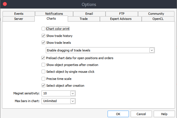
また、何らかの理由で履歴データを取得できない場合は、以下の手順でMetaTrader 5プラットフォーム上で手動で取得することが可能です。まず、MetaTraderプラットフォームを起動し、MetaTrader 5のペイン/パネル上部にある[ツール]>[オプション]に移動します。次に、チャートオプションのセクションに進みます。そこで、ダウンロードしたいチャートのバーの数を選択します。一定期間にどれだけのバーが存在するかは予測できないため、「無制限」のオプションを選択することをお勧めします。これにより、日付に基づいてデータを扱う際にも問題なく対応できます。
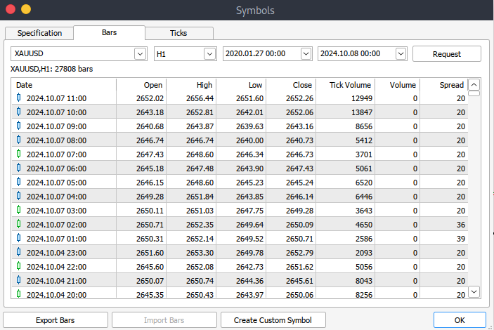
その後、実際のデータをダウンロードする必要があります。手順としては、[表示]>[銘柄]に進み、[仕様]タブに移動します。その後、ダウンロードしたいデータの種類に応じて、[Bars]または[Ticks]を選択します。次に、ダウンロードしたい履歴データの開始日と終了日を入力し、リクエストボタンをクリックします。これにより、データがダウンロードされ、.csv形式で保存されます。
Jupyter LabでのMetaTrader 5データの可視化
MetaTrader 5の履歴データをJupyter Labにロードするには、まずデータがダウンロードされたフォルダを見つける必要があります。Jupyter Labを開いたら、そのフォルダに移動してファイルにアクセスします。その後、データをロードし、列名を確認する手順に進みます。列名を確認することは、データを正しく管理し、不適切な列名の使用によるエラーを防ぐために重要です。
以下はPythonのコードです。
import pandas as pd

# assign variable to the historical data
file_path = '/home/int_junkie/Documents/ML/predi/XAUUSD.m_H1_2nd.csv'

data = pd.read_csv(file_path, delimiter='\t')

# Display the first few rows and column names
print(data.head())
print(data.columns)

過去のデータは2024年1月2日から現在のデータまでです。
以下はPythonのコードです。
# Convert the <DATE> and <TIME> columns into a single datetime column
data['<DATETIME>'] = pd.to_datetime(data['<DATE>'] + ' ' + data['<TIME>'], format='%Y.%m.%d %H:%M:%S')

# Drop the original <DATE> and <TIME> columns
data = data.drop(columns=['<DATE>', '<TIME>'])

# Convert numeric columns from strings to appropriate float types
numeric_columns = ['<OPEN>', '<HIGH>', '<LOW>', '<CLOSE>', '<TICKVOL>', '<VOL>', '<SPREAD>']
data[numeric_columns] = data[numeric_columns].apply(pd.to_numeric)

# Set datetime as index for easier plotting
data.set_index('<DATETIME>', inplace=True)

# Let's plot the close price and tick volume to visualize the trend
import matplotlib.pyplot as plt

# Plot closing price and tick volume
fig, ax1 = plt.subplots(figsize=(12, 6))

# Close price on primary y-axis
ax1.set_xlabel('Date')
ax1.set_ylabel('Close Price', color='tab:blue')
ax1.plot(data.index, data['<CLOSE>'], color='tab:blue', label='Close Price')
ax1.tick_params(axis='y', labelcolor='tab:blue')

# Tick volume on secondary y-axis
ax2 = ax1.twinx()
ax2.set_ylabel('Tick Volume', color='tab:green')
ax2.plot(data.index, data['<TICKVOL>'], color='tab:green', label='Tick Volume')
ax2.tick_params(axis='y', labelcolor='tab:green')

# Show the plot
plt.title('Close Price and Tick Volume Over Time')
fig.tight_layout()
plt.show()

上のプロットは、2つの主要指標を時系列で示しています。
- 終値(青):チャート上で各時間の終値を表しています。これにより、金価格(XAU/USD)の上昇トレンドや下降トレンドを含む経時的な変動を観察することができます。
- ティックボリューム(緑):各時間内の価格変動の回数を示しています。ティックボリュームの急上昇は、市場の活況やボラティリティの増加に関連していることが多いです。たとえば、ティックボリュームが高い時間帯は、大きな価格変動を伴い、重要なイベントや市場心理の変化を示唆する場合があります。
それでは、このデータをさらに詳しく掘り下げてみましょう。
1. トレンド分析
# Calculating moving averages: 50-period and 200-period for trend analysis
data['MA50'] = data['<CLOSE>'].rolling(window=50).mean()
data['MA200'] = data['<CLOSE>'].rolling(window=200).mean()

# Plot close price along with the moving averages
plt.figure(figsize=(12, 6))

# Plot close price
plt.plot(data.index, data['<CLOSE>'], label='Close Price', color='blue')

# Plot moving averages
plt.plot(data.index, data['MA50'], label='50-Period Moving Average', color='orange')
plt.plot(data.index, data['MA200'], label='200-Period Moving Average', color='red')

plt.title('Close Price with 50 & 200 Period Moving Averages')
plt.xlabel('Date')
plt.ylabel('Price')
plt.legend(loc='best')
plt.grid(True)
plt.show()
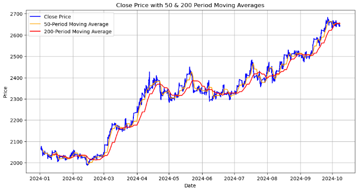
このプロットは、終値と50期間および200期間の移動平均線を示しています。
- 終値(青線):各期間の終了時点での実際の価格を表しています。
- 50期間移動平均線(オレンジ線):50期間の価格データを平滑化する短期移動平均線です。この線が終値より上にクロスした場合、上昇トレンドの可能性を示唆し、下にクロスした場合は下降トレンドの兆しとなります。
- 200期間移動平均線(赤線):長期的な移動平均線で、全体的な市場トレンドを把握するために使用します。価格変動に対して反応が遅いため、50期間移動平均線とのクロスオーバーは、長期的なトレンド反転を示す重要なシグナルとなります。
重要なポイントはゴールデンクロスであり、50期間の移動平均線が200期間の移動平均線を上回った場合、強気のトレンドが始まる可能性を示唆します。逆に、デッドクロスは50期間移動平均線が200期間移動平均線を下回る場合、弱気のトレンドを示唆することがあります。
次に、価格帯(高値と安値の差)を計算してボラティリティを分析し、それを可視化します。
2. ボラティリティ分析
# Calculate the price range (High - Low)
data['Price_Range'] = data['<HIGH>'] - data['<LOW>']

# Calculate Bollinger Bands
# Use a 20-period moving average and 2 standard deviations
data['MA20'] = data['<CLOSE>'].rolling(window=20).mean()
data['BB_upper'] = data['MA20'] + 2 * data['<CLOSE>'].rolling(window=20).std()
data['BB_lower'] = data['MA20'] - 2 * data['<CLOSE>'].rolling(window=20).std()

# Plot the price range and Bollinger Bands along with the close price
plt.figure(figsize=(12, 8))

# Plot the close price
plt.plot(data.index, data['<CLOSE>'], label='Close Price', color='blue')

# Plot Bollinger Bands
plt.plot(data.index, data['BB_upper'], label='Upper Bollinger Band', color='red', linestyle='--')
plt.plot(data.index, data['BB_lower'], label='Lower Bollinger Band', color='green', linestyle='--')

# Fill the area between Bollinger Bands for better visualization
plt.fill_between(data.index, data['BB_upper'], data['BB_lower'], color='gray', alpha=0.3)

# Plot the price range on a separate axis
plt.figure(figsize=(12, 6))
plt.plot(data.index, data['Price_Range'], label='Price Range (High-Low)', color='purple')

plt.title('Bollinger Bands and Price Range (Volatility Analysis)')
plt.xlabel('Date')
plt.ylabel('Price')
plt.legend(loc='best')
plt.grid(True)
plt.show()

上記の出力から、以下の内容を実行しました。
- 価格帯の計算:各時間帯の価格帯は、最高価格(<High>から最低価格(<LOW>)を引くことで計算されます。これは、各時間帯の値動きの程度を把握し、その時間帯のボラティリティを測定するのに役立ちます。
- `data['Price-Range'] = data['<HIGH>'] - data['<LOW>'] :その結果、Price-Range列には、各時間内で価格がどの程度変動したかが示されます。
- ボリンジャーバンドの計算:ボリンジャーバンドは、価格変動の程度に関する洞察を得るために計算されます。MA-20は終値の20期間移動平均です。ボリンジャーバンドの中間線の役割を果たします。BB-upperは上限バンド、BB-lowerは下限バンドを表します。これは、20期間の移動平均の上下にある2つの標準偏差として計算されます。価格が上限バンドに近づく場合、市場が買われすぎの可能性があることを示唆します。同様に、下限バンドに近づく場合、市場が売られすぎの可能性があることを示します。
- 価格とボリンジャーバンドの視覚化:終値(青線)は、各期間の実際の終値を示しています。上限ボリンジャーバンド(赤の破線)と下限ボリンジャーバンド(緑の破線)は、移動平均線の上下に形成されるボラティリティバンドを表しています。グレーの網掛け部分は、上限バンドと下限バンドに挟まれたエリアで、価格がこの範囲内で動くと予想されるボラティリティの幅を視覚的に表現しています。
- 価格帯別プロット:2つ目のプロットでは、ボラティリティの時間的な変動を別個に示しています。紫色の線で表された価格帯は、各時間内でのボラティリティの大きさを示します。このプロットにおける大きなスパイクは、ボラティリティが特に増加した期間を意味します。
import pandas as pd
import talib
from stable_baselines3 import DQN
from stable_baselines3.common.env_checker import check_env

# Verify the environment
check_env(env)

# Initialize and train the DQN model
model = DQN('MlpPolicy', env, verbose=1)
model.learn(total_timesteps=10000)

# Save the trained model
model.save("trading_dqn_model")

# Load and preprocess the data as before
data = pd.read_csv('XAUUSD_H1_Data-V.csv', delimiter='\t')
data['<DATETIME>'] = pd.to_datetime(data['<DATE>'] + ' ' + data['<TIME>'], format='%Y.%m.%d %H:%M:%S')
data = data.drop(columns=['<DATE>', '<TIME>'])
numeric_columns = ['<OPEN>', '<HIGH>', '<LOW>', '<CLOSE>', '<TICKVOL>', '<VOL>', '<SPREAD>']
data[numeric_columns] = data[numeric_columns].apply(pd.to_numeric)
data.set_index('<DATETIME>', inplace=True)

# Calculate Bollinger Bands (20-period moving average with 2 standard deviations)
data['MA20'] = data['<CLOSE>'].rolling(window=20).mean()
data['BB_upper'] = data['MA20'] + 2 * data['<CLOSE>'].rolling(window=20).std()
data['BB_lower'] = data['MA20'] - 2 * data['<CLOSE>'].rolling(window=20).std()

# Calculate percentage price change and volume change as additional features
data['Pct_Change'] = data['<CLOSE>'].pct_change()
data['Volume_Change'] = data['<VOL>'].pct_change()

# Fill missing values
data.fillna(0, inplace=True)
上記のコードでは、stable-baseline3のDQN (Deep Q-Network)アルゴリズムを使用して、XAU/USD(金)市場の取引決定を行う強化学習(RL)モデルのために金融データを準備しています。まず、過去のデータを読み込み処理し、ボリンジャーバンド(移動平均と価格のボラティリティに基づくテクニカル指標)を計算します。そして、価格や出来高の変化率などの特徴量を追加します。環境が検証され、DQNモデルは10,000タイムステップで訓練され、その後モデルは将来の使用のために保存されます。最後に、欠損データはゼロで埋められ、スムーズなモデル学習が可能となります。
import gym
from gym import spaces
import numpy as np

class TradingEnv(gym.Env):
    def __init__(self, data):
        super(TradingEnv, self).__init__()

        # Market data and feature columns
        self.data = data
        self.current_step = 0

        # Define action and observation space
        # Actions: 0 = Hold, 1 = Buy, 2 = Sell
        self.action_space = spaces.Discrete(3)

        # Observations (features: Bollinger Bands, Price Change, Volume Change)
        self.observation_space = spaces.Box(low=-np.inf, high=np.inf, shape=(5,), dtype=np.float32)

        # Initial balance and positions
        self.balance = 10000  # Starting balance
        self.position = 0  # No position at the start (0 = no trade, 1 = buy, -1 = sell)

    def reset(self):
        self.current_step = 0
        self.balance = 10000
        self.position = 0
        return self._next_observation()

    def _next_observation(self):
        # Get the current market data (Bollinger Bands, Price Change, Volume Change)
        obs = np.array([
            self.data['BB_upper'].iloc[self.current_step],
            self.data['BB_lower'].iloc[self.current_step],
            self.data['Pct_Change'].iloc[self.current_step],
            self.data['Volume_Change'].iloc[self.current_step],
            self.position
        ])
        return obs

    def step(self, action):
        # Execute the trade based on action and update balance and position
        self.current_step += 1

        # Get current price
        current_price = self.data['<CLOSE>'].iloc[self.current_step]

        reward = 0  # Reward initialization
        done = self.current_step == len(self.data) - 1  # Check if we're done

        # Buy action
        if action == 1 and self.position == 0:
            self.position = 1
            self.entry_price = current_price

        # Sell action
        elif action == 2 and self.position == 1:
            reward = current_price - self.entry_price
            self.balance += reward
            self.position = 0

        # Hold action
        else:
            reward = 0

        return self._next_observation(), reward, done, {}

    def render(self, mode='human', close=False):
        # Optional: Print the current balance and position
        print(f"Step: {self.current_step}, Balance: {self.balance}, Position: {self.position}")

# Create the trading environment
env = TradingEnv(data)
上記のコードでは、gymライブラリを使用して取引環境TradingEnvクラスを定義し、過去の市場データに基づいた取引環境をシミュレートしています。この環境では、ホールド、買い、売りの3つのアクションが可能です。観測空間には、5つの特徴量(ボリンジャーバンド、価格の変化率、出来高の変化率、現在の取引ポジション)が含まれています。エージェントは1万ユニットの残高とポジションなしの状態でスタートします。各ステップで、選択されたアクションに基づき、環境はエージェントのポジションと残高を更新し、利益のある取引に対して報酬を計算し、データの次のステップに進みます。環境はリセットして新しいエピソードを開始したり、取引プロセスの現在の状態をレンダリングすることも可能です。この環境は強化学習モデルの訓練に使用されます。
import gymnasium as gym
from gymnasium import spaces
import numpy as np
from stable_baselines3 import DQN
from stable_baselines3.common.env_checker import check_env

# Define the custom Trading Environment
class TradingEnv(gym.Env):
    def __init__(self, data):
        super(TradingEnv, self).__init__()

        # Market data and feature columns
        self.data = data
        self.current_step = 0

        # Define action and observation space
        # Actions: 0 = Hold, 1 = Buy, 2 = Sell
        self.action_space = spaces.Discrete(3)

        # Observations (features: Bollinger Bands, Price Change, Volume Change)
        self.observation_space = spaces.Box(low=-np.inf, high=np.inf, shape=(5,), dtype=np.float32)

        # Initial balance and positions
        self.balance = 10000  # Starting balance
        self.position = 0  # No position at the start (0 = no trade, 1 = buy, -1 = sell)

    def reset(self, seed=None, options=None):
        # Initialize the random seed
        self.np_random, seed = self.seed(seed)

        self.current_step = 0
        self.balance = 10000
        self.position = 0

        # Return initial observation and an empty info dictionary
        return self._next_observation(), {}

    def _next_observation(self):
        # Get the current market data (Bollinger Bands, Price Change, Volume Change)
        obs = np.array([
            self.data['BB_upper'].iloc[self.current_step],
            self.data['BB_lower'].iloc[self.current_step],
            self.data['Pct_Change'].iloc[self.current_step],
            self.data['Volume_Change'].iloc[self.current_step],
            self.position
        ], dtype=np.float32)  # Explicitly cast to float32
        return obs

    def step(self, action):
        self.current_step += 1
        current_price = self.data['<CLOSE>'].iloc[self.current_step]

        reward = 0
        done = self.current_step == len(self.data) - 1
        truncated = False  # Set to False unless there's an external condition to end the episode early

        # Execute the action
        if action == 1 and self.position == 0:
            self.position = 1
            self.entry_price = current_price

        elif action == 2 and self.position == 1:
            reward = current_price - self.entry_price
            self.balance += reward
            self.position = 0

        # Return next observation, reward, terminated, truncated, and an empty info dict
        return self._next_observation(), reward, done, truncated, {}

    def render(self, mode='human', close=False):
        print(f"Step: {self.current_step}, Balance: {self.balance}, Position: {self.position}")

    def seed(self, seed=None):
        self.np_random, seed = gym.utils.seeding.np_random(seed)
        return self.np_random, seed

# Assuming your data is already prepared (as a DataFrame) and includes Bollinger Bands and other necessary features
# Create the environment
env = TradingEnv(data)

# Verify the environment
check_env(env)

# Train the model using DQN
model = DQN('MlpPolicy', env, verbose=1)
model.learn(total_timesteps=10000)

# Save the trained model
model.save("trading_dqn_model")
以下は出力です。

次に、強化学習のためにgymnasiumを使用して、エージェントが過去の市場データに基づいて取引決定を学習するカスタム取引環境を定義します。 この環境では、ホールド、買い、売りの3つのアクションが可能で、ボリンジャーバンド、価格変化率、出来高変化率、現在のポジションなどの5つの観測が含まれています。エージェントは1万ドルの残高があり、未決済のポジションがない状態からスタートします。環境内の各ステップはエージェントを前進させ、その位置、バランスを更新し、成功した取引の報酬を計算します。環境はstable-baseline3のcheck-Env()関数を使って検証され、DQN (Deep Q-Network)モデルは最適な取引戦略を学習するために10,000タイムステップ学習されます。学習されたモデルは、将来自動売買システムで使用するために保存されます。
# Unpack the observation from the reset() method
obs, _ = env.reset()

# Loop through the environment steps
for step in range(len(data)):
    # Predict the action based on the observation
    action, _states = model.predict(obs)

    # Step the environment
    obs, rewards, done, truncated, info = env.step(action)

    # Render the environment (print the current state)
    env.render()

    # Check if the episode is done
    if done or truncated:
        print("Testing completed!")
        break


その結果、学習済みモデルによって実行された取引戦略は取引期間中にわずかな利益をもたらし、残高は10,000ドルから10,108ドルに増加しました。これは、モデルが利益の出る取引を特定できたことを示唆していますが、108ドル(1.08%の利益)という利益率は比較的控えめです。
この結果は、モデルが慎重または低頻度の取引を行っていることを示唆するか、あるいは戦略がより高いリターンを得るために十分に最適化されていないことを示している可能性があります。さらに長期間のテストや、モデルパラメータ(報酬関数、特徴選択、取引実行ロジックなど)の調整を含む評価が、モデルのパフォーマンス向上に役立つ可能性があります。また、取引コストやリスク管理などの要因を考慮して、戦略が長期的に利益を確保できることが重要です。
MQL5ですべてをまとめる
MQL5を学習済みモデルを実行するPythonスクリプトに接続するためには、MQL5とPython間の通信チャネルを設定する必要があります。ここでは、一般的に使用されるソケットサーバを利用します。//+------------------------------------------------------------------+ //| EnhancedML.mq5 | //| Copyright 2024, MetaQuotes Ltd. | //| https://www.mql5.com | //+------------------------------------------------------------------+ #property copyright "Copyright 2024, MetaQuotes Ltd." #property link "https://www.mql5.com" #property version "1.00" //+------------------------------------------------------------------+ //| Includes | //+------------------------------------------------------------------+ #include <WinAPI\winapi.mqh> #include <Trade\Trade.mqh> CTrade trade;
まず、システムレベルの操作のためのWindows APIライブラリ(winapi.mqh)と、取引管理のための取引ライブラリ(trade.mqh)が含まれています。次にCTradeクラスのインスタンスをtradeと名付け宣言します。
//+------------------------------------------------------------------+
//|                          Global Vars                             |
//+------------------------------------------------------------------+
int stopLoss = 350;
int takeProfit = 500;

string Address = "127.0.0.1";
int port = 9999;
int socket = SocketCreate();

double Bid = SymbolInfoDouble(_Symbol, SYMBOL_BID);
double Ask = SymbolInfoDouble(_Symbol, SYMBOL_ASK);
Addressを127.0.0.1(ローカルホスト)に、portをソケット通信に使用する9999に設定します。SocketCreate()関数はソケットを初期化してsocket変数にソケットハンドルを格納し、Pythonサーバとの通信を可能にします。
//+------------------------------------------------------------------+
//| Expert initialization function                                   |
//+------------------------------------------------------------------+
int OnInit(){

    if (!SocketConnect(socket, Address, port, 1000)){
        Print("Successfully connected to ", Address, ":", port);
    } else {
        Print("Connection to ", Address, ":", port, " failed, error ", GetLastError());
        return INIT_FAILED;
    }

   return(INIT_SUCCEEDED);
}
SocketConnect()関数は、作成したソケットを、与えられたアドレス(ローカルホスト)とポート9999にあるPythonサーバに接続しようとします。ミリ秒単位のタイムアウトは1000です。
//+------------------------------------------------------------------+
//| Expert tick function                                             |
//+------------------------------------------------------------------+
void OnTick(){


   uint len=SocketIsReadable(socket);

   char buffer[16];
   int bytes = SocketRead(socket, buffer, len, 23);

   if (bytes > 0){

      string action_str = CharArrayToString(buffer);

      int action = StringToInteger(action_str);
      //int action = atoi(buffer);

      // Execute a trade based on action
      if(action == 1){
         //buy trade
         MBuy();
         Print("Buy action received...");
      } else if(action == 2){
         //sell trade
         MSell();
         Print("Sell action received...");
      }
   }

}
MQL5のOnTick()関数は、ソケット接続を通じて各マーケットティックで受信した取引指示を処理するように設計されています。まず、SocketIsReadable()を使用してソケットにデータがあるか確認し、データの長さを返します。データが存在する場合、SocketRead()関数でデータをバッファに読み込み、読み込んだバイト数をbytesに格納します。データを受信した後、バッファは文字列に変換され、その後整数(action)に変換されます。actionの値に基づいて、この関数は対応する取引を実行します。action == 1の場合はMBuy()を呼び出して買い取引を実行し、action == 2の場合はMSell()を呼び出して売り取引を実行します。各取引アクション後にprint文が受け取ったアクション(買いまたは売り)をログに記録します。要するに、この関数はソケット経由で売買コマンドを受信し、それに応じて自動的に取引を実行します。
//+------------------------------------------------------------------+
//|                        Buy Function                              |
//+------------------------------------------------------------------+
void MBuy(){

   static int digits = (int)SymbolInfoInteger(_Symbol, SYMBOL_DIGITS);

   double Lots = 0.02;
   double sl = NormalizeDouble(SymbolInfoDouble(_Symbol, SYMBOL_BID) - stopLoss, digits);
   double tp = NormalizeDouble(SymbolInfoDouble(_Symbol,SYMBOL_ASK) + takeProfit * _Point, digits);
   trade.PositionOpen(_Symbol, ORDER_TYPE_BUY, Lots, Ask, sl, tp);
}
以下は、買い取引を開始する関数です。
//+------------------------------------------------------------------+
//|                         Sell Function                            |
//+------------------------------------------------------------------+
void MSell(){
   static int digits = (int)SymbolInfoInteger(_Symbol, SYMBOL_DIGITS);

   double Lots = 0.02;
   double sl = NormalizeDouble(SymbolInfoDouble(_Symbol, SYMBOL_ASK) + stopLoss, digits);
   double tp = NormalizeDouble(SymbolInfoDouble(_Symbol,SYMBOL_BID) - takeProfit * _Point, digits);
   trade.PositionOpen(_Symbol, ORDER_TYPE_SELL, Lots, Bid, sl, tp);
}
以下は、売り取引を開始する関数です。
Pythonソケットサーバスクリプト(取引モデルサーバ)
Pythonスクリプトは学習済みモデルをロードし、MQL5からの接続をリッスンするソケットサーバをセットアップします。データを受信すると、予測を立て、取引アクションを送り返します。
import socket
import numpy as np
from stable_baselines3 import DQN

# Load the trained model
model = DQN.load("trading_dqn_model")

# Set up the server
HOST = '127.0.0.1'  # Localhost (you can replace this with your IP)
PORT = 9999         # Port to listen on

# Create a TCP/IP socket
server_socket = socket.socket(socket.AF_INET, socket.SOCK_STREAM)
server_socket.bind((HOST, PORT))
server_socket.listen(1)

print(f"Server listening on {HOST}:{PORT}...")

while True:
    # Wait for a connection
    client_socket, client_address = server_socket.accept()
    print(f"Connection from {client_address}")

    # Receive data from MQL5 (price data sent by EA)
    data = client_socket.recv(1024).decode('utf-8')

    if data:
        print(f"Received data: {data}")

        # Convert received data to a numpy array
        observation = np.fromstring(data, sep=',')  # Assumes comma-separated price data

        # Make prediction using the model
        action, _ = model.predict(observation)

        # Send the predicted action back to MQL5
        client_socket.send(str(action).encode('utf-8'))

    # Close the client connection
    client_socket.close()
Pythonスクリプトをtrading-model-server.pyまたは任意の名前で保存します。端末かコマンドプロンプトを開き、モデルを保存したディレクトリとtrading-model-server.pyに移動し、以下を実行して接続を確立します。
python trading_model_server.py
結論
まとめると、私たちは機械学習とMQL5を統合し、過去のデータに基づいて取引判断を自動化する包括的な取引システムを開発しました。最初にXAU/USDの履歴データを読み込み、前処理を行い、ボリンジャーバンドを計算し、価格や出来高の変化といったその他の主要な特徴を実装しました。次に、強化学習、特にDeep Q-Network (DQN)を使用して、データのパターンに基づいて売買アクションを予測するモデルを訓練しました。訓練されたモデルはソケット通信システムを通じてMQL5に接続され、取引プラットフォームとPythonベースの意思決定モデルの間でリアルタイムのやり取りが可能となりました。これにより、モデルの予測に基づいて取引が自動的に実行され、システム全体がアルゴリズム取引の強力なツールとなりました。
データの可視化と機械学習の統合を強化することで、トレーダーにより深い洞察と情報に基づいた意思決定を提供し、大きな利益をもたらすことができます。市場のトレンド、ボラティリティ、主要なパターンを分析することで、システムは取引の最適なエントリーポイントとエグジットポイントを特定できます。データ駆動型モデルに基づく取引執行の自動化により、人的エラーや感情的バイアスが減少し、より一貫性のある戦略的な取引が可能になります。全体として、このアプローチはトレーダーに過去のデータを活用してパフォーマンスを向上させる洗練されたツールを提供し、反復的な取引作業を自動化することで時間を節約します。
MetaQuotes Ltdにより英語から翻訳されました。
元の記事: https://www.mql5.com/en/articles/16083
警告: これらの資料についてのすべての権利はMetaQuotes Ltd.が保有しています。これらの資料の全部または一部の複製や再プリントは禁じられています。
この記事はサイトのユーザーによって執筆されたものであり、著者の個人的な見解を反映しています。MetaQuotes Ltdは、提示された情報の正確性や、記載されているソリューション、戦略、または推奨事項の使用によって生じたいかなる結果についても責任を負いません。

- 無料取引アプリ
- 8千を超えるシグナルをコピー
- 金融ニュースで金融マーケットを探索
mt5からpythonにデータを送る場所はどこですか?
コードを実行したわけではないのですが、どうも足りないようです。
mt5からpythonにデータを送る場所は?
コードを実行したわけではないのですが、どうも足りないようです。