
将 MQL5 与数据处理包集成(第 3 部分):增强的数据可视化

概述
金融市场的交易者经常面临理解大量数据的挑战,从价格波动和交易量到技术指标和经济新闻。随着现代市场的速度和复杂性,使用传统方法有效地解释这些数据流变得越来越困难。仅凭图表可能无法提供足够的洞察力,导致错失机会或做出不合时宜的决定。快速识别趋势、逆转和潜在风险的需要增加了难度。对于希望做出明智、数据驱动决策的交易者来说,无法从数据中提取关键见解是一个关键问题,可能会导致利润损失或风险增加。
增强的数据可视化通过将原始金融数据转换为更直观和交互式的视觉表示来解决这一挑战。动态蜡烛图、技术指标叠加图和回报热图等工具为交易者提供了对市场状况更深入、更可行的理解。通过整合突出趋势、相关性和异常的视觉元素,交易者可以快速发现机会并做出更明智的决策。这种增强的方法有助于降低解释数据的复杂性,使交易者能够在快速发展的金融市场中更加自信和高效地行事。
收集历史数据
from datetime import datetime
import MetaTrader5 as mt5
import pandas as pd
import pytz

# Display data on the MetaTrader 5 package
print("MetaTrader5 package author: ", mt5.__author__)
print("MetaTrader5 package version: ", mt5.__version__)

# Configure pandas display options
pd.set_option('display.max_columns', 500)
pd.set_option('display.width', 1500)

# Establish connection to MetaTrader 5 terminal
if not mt5.initialize():
    print("initialize() failed, error code =", mt5.last_error())
    quit()

# Set time zone to UTC
timezone = pytz.timezone("Etc/UTC")
# Create 'datetime' objects in UTC time zone to avoid the implementation of a local time zone offset
utc_from = datetime(2024, 1, 2, tzinfo=timezone)
utc_to = datetime.now(timezone)  # Set to the current date and time

# Get bars from XAUUSD H1 (hourly timeframe) within the specified interval
rates = mt5.copy_rates_range("XAUUSD", mt5.TIMEFRAME_H1, utc_from, utc_to)

# Shut down connection to the MetaTrader 5 terminal
mt5.shutdown()

# Check if data was retrieved
if rates is None or len(rates) == 0:
    print("No data retrieved. Please check the symbol or date range.")
else:
    # Display each element of obtained data in a new line (for the first 10 entries)
    print("Display obtained data 'as is'")
    for rate in rates[:10]:
        print(rate)

    # Create DataFrame out of the obtained data
    rates_frame = pd.DataFrame(rates)
    # Convert time in seconds into the 'datetime' format
    rates_frame['time'] = pd.to_datetime(rates_frame['time'], unit='s')

    # Save the data to a CSV file
    filename = "XAUUSD_H1_2nd.csv"
    rates_frame.to_csv(filename, index=False)
    print(f"\nData saved to file: {filename}")
为了检索历史数据,我们首先使用 “mt5.initialize()” 函数建立与 MetaTrader 5 终端的连接。这是必不可少的,因为 Python 包直接与正在运行的 MetaTrader 5 平台通信。我们通过指定开始和结束日期来配置代码,以设置数据提取所需的时间范围。`datetime` 对象是在 UTC 时区创建的,以确保跨不同时区的一致性。然后,脚本使用 `mt5.copy-rates-range()` 函数请求 XAUUSD 交易品种的历史小时数据,从 2024 年 1 月 2 日开始到当前日期和时间。
获取历史数据后,我们使用 “mt5.shutdown()” 安全地断开与 MetaTrader 5 终端的连接,以避免任何进一步的不必要的连接。获取到的数据最初以原始格式显示,以确认数据提取成功。我们将这些数据转换为 pandas DataFrame 以便于操作和分析。此外,该代码将 Unix 时间戳转换为可读的日期时间格式,确保数据结构良好,可供进一步处理或分析。这种方法允许交易者分析历史市场走势,并根据过去的表现做出明智的交易决策。
filename = "XAUUSD_H1_2nd.csv"
rates_frame.to_csv(filename, index=False)
print(f"\nData saved to file: {filename}")
由于我的操作系统是 Linux,我必须将收到的数据保存到一个文件中。但对于那些使用 Windows 的人来说,您只需使用以下脚本即可检索数据:
from datetime import datetime
import MetaTrader5 as mt5
import pandas as pd
import pytz

# Display data on the MetaTrader 5 package
print("MetaTrader5 package author: ", mt5.__author__)
print("MetaTrader5 package version: ", mt5.__version__)

# Configure pandas display options
pd.set_option('display.max_columns', 500)
pd.set_option('display.width', 1500)

# Establish connection to MetaTrader 5 terminal
if not mt5.initialize():
    print("initialize() failed, error code =", mt5.last_error())
    quit()

# Set time zone to UTC
timezone = pytz.timezone("Etc/UTC")
# Create 'datetime' objects in UTC time zone to avoid the implementation of a local time zone offset
utc_from = datetime(2024, 1, 2, tzinfo=timezone)
utc_to = datetime.now(timezone)  # Set to the current date and time

# Get bars from XAUUSD H1 (hourly timeframe) within the specified interval
rates = mt5.copy_rates_range("XAUUSD", mt5.TIMEFRAME_H1, utc_from, utc_to)

# Shut down connection to the MetaTrader 5 terminal
mt5.shutdown()

# Check if data was retrieved
if rates is None or len(rates) == 0:
    print("No data retrieved. Please check the symbol or date range.")
else:
    # Display each element of obtained data in a new line (for the first 10 entries)
    print("Display obtained data 'as is'")
    for rate in rates[:10]:
        print(rate)

    # Create DataFrame out of the obtained data
    rates_frame = pd.DataFrame(rates)
    # Convert time in seconds into the 'datetime' format
    rates_frame['time'] = pd.to_datetime(rates_frame['time'], unit='s')

    # Display data directly
    print("\nDisplay dataframe with data")
    print(rates_frame.head(10))
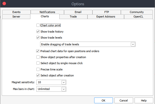
如果由于某种原因,您无法获取历史数据,您可以通过以下步骤在 MetTrader5 平台上手动检索。启动您的 MetaTrader 平台,在 MetaTrader 5 窗格/面板顶部导航至 >工具,然后 >选项,您将进入图表选项。然后您必须选择要下载的图表中的柱形数量。最好选择无限柱形的选项,因为我们将处理日期,并且我们不知道在给定的时间段内有多少柱形。
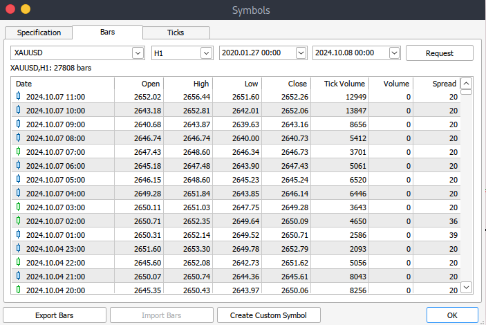
之后,您现在必须下载实际数据。为此,您必须导航至 >查看,然后导航至 >交易品种,然后进入规格选项卡。根据要下载的数据类型,只需导航至 > 柱或报价 。继续并输入您想要下载的历史数据的开始和结束日期,然后单击请求按钮下载数据并将其保存为 .csv 格式。
Jupyter Lab 上的 MetaTrader 5 数据可视化
要将 MetaTrader 5 历史数据加载到 Jupyter Lab 中,您首先需要找到下载数据的文件夹。进入 Jupyter Lab 后,导航到该文件夹以访问文件。下一步是加载数据并查看列名。检查列名对于确保正确管理数据并防止使用不正确的列名可能发生的错误非常重要。
Python 代码:
import pandas as pd

# assign variable to the historical data
file_path = '/home/int_junkie/Documents/ML/predi/XAUUSD.m_H1_2nd.csv'

data = pd.read_csv(file_path, delimiter='\t')

# Display the first few rows and column names
print(data.head())
print(data.columns)
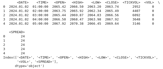
我们的历史数据从 2024 年 1 月 2 日开始,直到当前数据。
Python 代码:
# Convert the <DATE> and <TIME> columns into a single datetime column
data['<DATETIME>'] = pd.to_datetime(data['<DATE>'] + ' ' + data['<TIME>'], format='%Y.%m.%d %H:%M:%S')

# Drop the original <DATE> and <TIME> columns
data = data.drop(columns=['<DATE>', '<TIME>'])

# Convert numeric columns from strings to appropriate float types
numeric_columns = ['<OPEN>', '<HIGH>', '<LOW>', '<CLOSE>', '<TICKVOL>', '<VOL>', '<SPREAD>']
data[numeric_columns] = data[numeric_columns].apply(pd.to_numeric)

# Set datetime as index for easier plotting
data.set_index('<DATETIME>', inplace=True)

# Let's plot the close price and tick volume to visualize the trend
import matplotlib.pyplot as plt

# Plot closing price and tick volume
fig, ax1 = plt.subplots(figsize=(12, 6))

# Close price on primary y-axis
ax1.set_xlabel('Date')
ax1.set_ylabel('Close Price', color='tab:blue')
ax1.plot(data.index, data['<CLOSE>'], color='tab:blue', label='Close Price')
ax1.tick_params(axis='y', labelcolor='tab:blue')

# Tick volume on secondary y-axis
ax2 = ax1.twinx()
ax2.set_ylabel('Tick Volume', color='tab:green')
ax2.plot(data.index, data['<TICKVOL>'], color='tab:green', label='Tick Volume')
ax2.tick_params(axis='y', labelcolor='tab:green')

# Show the plot
plt.title('Close Price and Tick Volume Over Time')
fig.tight_layout()
plt.show()

上图显示了随时间变化的两个关键指标:
- 收盘价(蓝色):这代表图表上每小时的收盘价。我们可以观察到随时间推移的波动,表明黄金价格(XAU/USD)存在上涨和下跌趋势。
- 分时交易量(绿色):这表示每小时内价格变化的次数。分时交易量的飙升通常对应于市场活动或波动性的增加。例如,高交易量时期可能与重大价格变动相吻合,这可能预示着重要事件或市场情绪的转变。
现在让我们更深入地研究我们的数据:
1.趋势分析。
# Calculating moving averages: 50-period and 200-period for trend analysis
data['MA50'] = data['<CLOSE>'].rolling(window=50).mean()
data['MA200'] = data['<CLOSE>'].rolling(window=200).mean()

# Plot close price along with the moving averages
plt.figure(figsize=(12, 6))

# Plot close price
plt.plot(data.index, data['<CLOSE>'], label='Close Price', color='blue')

# Plot moving averages
plt.plot(data.index, data['MA50'], label='50-Period Moving Average', color='orange')
plt.plot(data.index, data['MA200'], label='200-Period Moving Average', color='red')

plt.title('Close Price with 50 & 200 Period Moving Averages')
plt.xlabel('Date')
plt.ylabel('Price')
plt.legend(loc='best')
plt.grid(True)
plt.show()
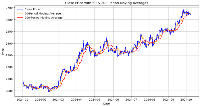
该图显示了收盘价以及 50 周期和 200 周期移动平均线:
- 收盘价(蓝色线):这代表了每个时间段结束时的实际价格。
- 50 周期移动平均线(橙色线):一个短期移动平均线,平滑了 50 个时期的价格数据。当收盘价越过这条线时,它可能预示着潜在的上涨趋势,当它穿过这条线以下时,可能预示着下跌趋势。
- 200 周期移动平均线(红色线):长期移动平均线,提供对整体趋势的洞察。它对价格变化的反应往往较慢,因此与 50 期移动平均线的交叉可能预示着长期趋势的重大逆转。
我们正在寻找的关键点是金叉,当 50 期移动平均线越过 200 期移动平均线上时,它可能预示着潜在的强劲看涨趋势。最后一个是死叉,当 50 期移动平均线穿过 200 期移动平均线上时,它可能预示着潜在的看跌趋势。
接下来,我们通过计算价格范围(最高价和最低价之间的差异)来分析波动性并将其可视化。
2.波动性分析。
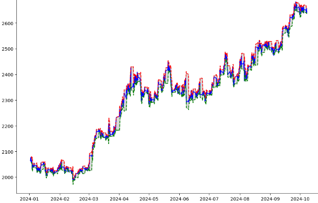
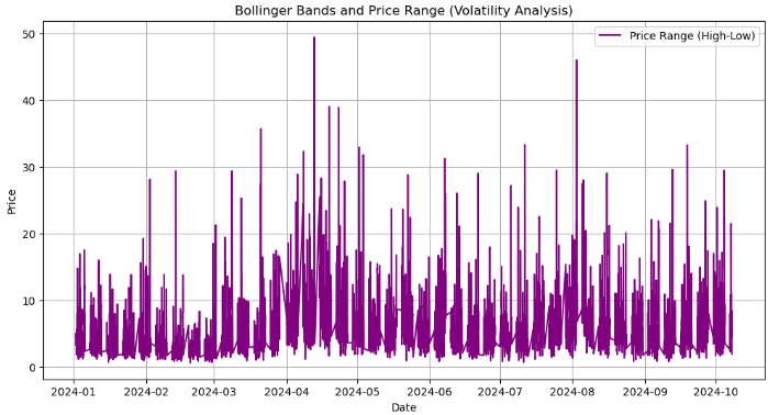
# Calculate the price range (High - Low)
data['Price_Range'] = data['<HIGH>'] - data['<LOW>']

# Calculate Bollinger Bands
# Use a 20-period moving average and 2 standard deviations
data['MA20'] = data['<CLOSE>'].rolling(window=20).mean()
data['BB_upper'] = data['MA20'] + 2 * data['<CLOSE>'].rolling(window=20).std()
data['BB_lower'] = data['MA20'] - 2 * data['<CLOSE>'].rolling(window=20).std()

# Plot the price range and Bollinger Bands along with the close price
plt.figure(figsize=(12, 8))

# Plot the close price
plt.plot(data.index, data['<CLOSE>'], label='Close Price', color='blue')

# Plot Bollinger Bands
plt.plot(data.index, data['BB_upper'], label='Upper Bollinger Band', color='red', linestyle='--')
plt.plot(data.index, data['BB_lower'], label='Lower Bollinger Band', color='green', linestyle='--')

# Fill the area between Bollinger Bands for better visualization
plt.fill_between(data.index, data['BB_upper'], data['BB_lower'], color='gray', alpha=0.3)

# Plot the price range on a separate axis
plt.figure(figsize=(12, 6))
plt.plot(data.index, data['Price_Range'], label='Price Range (High-Low)', color='purple')

plt.title('Bollinger Bands and Price Range (Volatility Analysis)')
plt.xlabel('Date')
plt.ylabel('Price')
plt.legend(loc='best')
plt.grid(True)
plt.show()
从上面的输出中,我们完成了以下工作:
- 价格范围计算:我们通过从最高价格(“ <High> ”)中减去最低价格(“ <LOW> ”)来计算每个时间段的价格范围。这给出了每个小时价格变动的程度,有助于衡量该时期的波动性。
- `data['Price-Range'] = data['<HIGH>'] - data['<LOW>'] :生成的 “Price-Rang”(价格范围)列显示了每小时内价格波动的幅度。
- 布林带计算:布林带指标是通过计算来了解价格波动的。` MA-20 ` 是收盘价的 20 周期移动平均线。它是布林带的中线。`BB-upper` 和 `BB-lower` 分别代表上轨和下轨。它们以 20 周期移动平均线的上下两个标准差来计算。当价格朝上轨移动时,表明市场可能超买;同样,朝下轨移动则表明市场可能超卖。
- 价格和布林带的可视化:收盘价(蓝色线),表示每个时间段的实际收盘价。上布林带(红色虚线)和下布林带(绿色虚线),这些线显示了围绕移动平均线形成布林带的波动带。阴影区域,布林带上下轨之间的区域呈灰色阴影,直观地表示价格预期波动的范围。
- 单独价格范围图:第二张图将价格范围显示为一条单独的紫色线,显示波动率随时间的变化情况。该图中较大的峰值表明波动性增加的时期。
import pandas as pd
import talib
from stable_baselines3 import DQN
from stable_baselines3.common.env_checker import check_env

# Verify the environment
check_env(env)

# Initialize and train the DQN model
model = DQN('MlpPolicy', env, verbose=1)
model.learn(total_timesteps=10000)

# Save the trained model
model.save("trading_dqn_model")

# Load and preprocess the data as before
data = pd.read_csv('XAUUSD_H1_Data-V.csv', delimiter='\t')
data['<DATETIME>'] = pd.to_datetime(data['<DATE>'] + ' ' + data['<TIME>'], format='%Y.%m.%d %H:%M:%S')
data = data.drop(columns=['<DATE>', '<TIME>'])
numeric_columns = ['<OPEN>', '<HIGH>', '<LOW>', '<CLOSE>', '<TICKVOL>', '<VOL>', '<SPREAD>']
data[numeric_columns] = data[numeric_columns].apply(pd.to_numeric)
data.set_index('<DATETIME>', inplace=True)

# Calculate Bollinger Bands (20-period moving average with 2 standard deviations)
data['MA20'] = data['<CLOSE>'].rolling(window=20).mean()
data['BB_upper'] = data['MA20'] + 2 * data['<CLOSE>'].rolling(window=20).std()
data['BB_lower'] = data['MA20'] - 2 * data['<CLOSE>'].rolling(window=20).std()

# Calculate percentage price change and volume change as additional features
data['Pct_Change'] = data['<CLOSE>'].pct_change()
data['Volume_Change'] = data['<VOL>'].pct_change()

# Fill missing values
data.fillna(0, inplace=True)
在上面的代码中,我们为强化学习(RL)模型准备财务数据,以便使用来自 “stable-baseline3” 的DQN(深度 Q 网络)算法对 XAU / USD(黄金)市场做出交易决策。它首先加载和处理历史数据,包括计算布林带(基于移动平均线和价格波动的技术指标)并添加百分比价格和交易量变化等功能。环境经过验证,并对 DQN 模型进行了 10000 个时间步的训练,之后保存该模型以供将来使用。最后,用零填充缺失的数据,以确保模型训练的顺利进行。
import gym
from gym import spaces
import numpy as np

class TradingEnv(gym.Env):
    def __init__(self, data):
        super(TradingEnv, self).__init__()

        # Market data and feature columns
        self.data = data
        self.current_step = 0

        # Define action and observation space
        # Actions: 0 = Hold, 1 = Buy, 2 = Sell
        self.action_space = spaces.Discrete(3)

        # Observations (features: Bollinger Bands, Price Change, Volume Change)
        self.observation_space = spaces.Box(low=-np.inf, high=np.inf, shape=(5,), dtype=np.float32)

        # Initial balance and positions
        self.balance = 10000  # Starting balance
        self.position = 0  # No position at the start (0 = no trade, 1 = buy, -1 = sell)

    def reset(self):
        self.current_step = 0
        self.balance = 10000
        self.position = 0
        return self._next_observation()

    def _next_observation(self):
        # Get the current market data (Bollinger Bands, Price Change, Volume Change)
        obs = np.array([
            self.data['BB_upper'].iloc[self.current_step],
            self.data['BB_lower'].iloc[self.current_step],
            self.data['Pct_Change'].iloc[self.current_step],
            self.data['Volume_Change'].iloc[self.current_step],
            self.position
        ])
        return obs

    def step(self, action):
        # Execute the trade based on action and update balance and position
        self.current_step += 1

        # Get current price
        current_price = self.data['<CLOSE>'].iloc[self.current_step]

        reward = 0  # Reward initialization
        done = self.current_step == len(self.data) - 1  # Check if we're done

        # Buy action
        if action == 1 and self.position == 0:
            self.position = 1
            self.entry_price = current_price

        # Sell action
        elif action == 2 and self.position == 1:
            reward = current_price - self.entry_price
            self.balance += reward
            self.position = 0

        # Hold action
        else:
            reward = 0

        return self._next_observation(), reward, done, {}

    def render(self, mode='human', close=False):
        # Optional: Print the current balance and position
        print(f"Step: {self.current_step}, Balance: {self.balance}, Position: {self.position}")

# Create the trading environment
env = TradingEnv(data)
从上面的代码中,我们使用 `gym` 库定义了一个交易环境 `TradingEnv` 类,以根据历史市场数据模拟交易环境。环境允许三种可能的操作:持有、买入或卖出。它包括一个具有五个特征(布林带、百分比价格变化、交易量变化和当前交易头寸)的观察空间。代理开始时余额为 10000 个单位且无头寸。在每一步中,基于所选操作,环境更新代理的位置和余额,计算盈利交易的奖励,并前进到数据中的下一步。环境可以重置以开始新的事件或呈现交易过程的当前状态。该环境将用于训练强化学习模型。
import gymnasium as gym
from gymnasium import spaces
import numpy as np
from stable_baselines3 import DQN
from stable_baselines3.common.env_checker import check_env

# Define the custom Trading Environment
class TradingEnv(gym.Env):
    def __init__(self, data):
        super(TradingEnv, self).__init__()

        # Market data and feature columns
        self.data = data
        self.current_step = 0

        # Define action and observation space
        # Actions: 0 = Hold, 1 = Buy, 2 = Sell
        self.action_space = spaces.Discrete(3)

        # Observations (features: Bollinger Bands, Price Change, Volume Change)
        self.observation_space = spaces.Box(low=-np.inf, high=np.inf, shape=(5,), dtype=np.float32)

        # Initial balance and positions
        self.balance = 10000  # Starting balance
        self.position = 0  # No position at the start (0 = no trade, 1 = buy, -1 = sell)

    def reset(self, seed=None, options=None):
        # Initialize the random seed
        self.np_random, seed = self.seed(seed)

        self.current_step = 0
        self.balance = 10000
        self.position = 0

        # Return initial observation and an empty info dictionary
        return self._next_observation(), {}

    def _next_observation(self):
        # Get the current market data (Bollinger Bands, Price Change, Volume Change)
        obs = np.array([
            self.data['BB_upper'].iloc[self.current_step],
            self.data['BB_lower'].iloc[self.current_step],
            self.data['Pct_Change'].iloc[self.current_step],
            self.data['Volume_Change'].iloc[self.current_step],
            self.position
        ], dtype=np.float32)  # Explicitly cast to float32
        return obs

    def step(self, action):
        self.current_step += 1
        current_price = self.data['<CLOSE>'].iloc[self.current_step]

        reward = 0
        done = self.current_step == len(self.data) - 1
        truncated = False  # Set to False unless there's an external condition to end the episode early

        # Execute the action
        if action == 1 and self.position == 0:
            self.position = 1
            self.entry_price = current_price

        elif action == 2 and self.position == 1:
            reward = current_price - self.entry_price
            self.balance += reward
            self.position = 0

        # Return next observation, reward, terminated, truncated, and an empty info dict
        return self._next_observation(), reward, done, truncated, {}

    def render(self, mode='human', close=False):
        print(f"Step: {self.current_step}, Balance: {self.balance}, Position: {self.position}")

    def seed(self, seed=None):
        self.np_random, seed = gym.utils.seeding.np_random(seed)
        return self.np_random, seed

# Assuming your data is already prepared (as a DataFrame) and includes Bollinger Bands and other necessary features
# Create the environment
env = TradingEnv(data)

# Verify the environment
check_env(env)

# Train the model using DQN
model = DQN('MlpPolicy', env, verbose=1)
model.learn(total_timesteps=10000)

# Save the trained model
model.save("trading_dqn_model")
输出:

然后,我们使用 “gymnasium” 来定义一个自定义交易环境进行强化学习,其中代理学习根据历史市场数据做出交易决策。该环境允许三种操作:持有、买入或卖出,并具有五种观察功能,包括布林带、百分比价格变化、成交量变化和当前仓位。代理商的起始余额为 10,000,并且没有未平仓头寸。环境中的每一步都会推动代理前进,更新其仓位、余额,并计算成功交易的奖励。使用 “stable-baseline3” 中的 “check-Env()” 函数验证环境,并对 DQN(深度 Q 网络)模型进行 10,000 个时间步长的训练,以学习最佳交易策略。训练好的模型被保存以供将来在自动交易系统中使用。
# Unpack the observation from the reset() method
obs, _ = env.reset()

# Loop through the environment steps
for step in range(len(data)):
    # Predict the action based on the observation
    action, _states = model.predict(obs)

    # Step the environment
    obs, rewards, done, truncated, info = env.step(action)

    # Render the environment (print the current state)
    env.render()

    # Check if the episode is done
    if done or truncated:
        print("Testing completed!")
        break


结果表明,训练模型实施的交易策略在交易期间带来了小幅盈利,余额从 10,000 美元增加到 10,108 美元。虽然这表明该模型能够识别有利可图的交易,但 108 美元的利润率(1.08% 的收益)相对较低。
结果表明,该模型正在进行谨慎或低频交易,或者可能表明该策略没有完全优化以获得更高的回报。进一步的评估,包括更长的测试期或对模型参数(如奖励函数、特征选择或交易执行逻辑)的调整,可以帮助提高模型的性能。考虑交易成本和风险管理等因素也很重要,以确保该策略随着时间的推移保持盈利。
将所有内容放在 MQL5 中
我们将把 MQL5 连接到将运行我们训练的模型的 Python 脚本,我们必须在 MQL5 和 Python 之间建立一个通信渠道。在我们的例子中,我们将使用一个常用的套接字服务器。//+------------------------------------------------------------------+ //| EnhancedML.mq5 | //| Copyright 2024, MetaQuotes Ltd. | //| https://www.mql5.com | //+------------------------------------------------------------------+ #property copyright "Copyright 2024, MetaQuotes Ltd." #property link "https://www.mql5.com" #property version "1.00" //+------------------------------------------------------------------+ //| Includes | //+------------------------------------------------------------------+ #include <WinAPI\winapi.mqh> #include <Trade\Trade.mqh> CTrade trade;
首先,我们包括用于系统级操作的 Windows API 库(“winapi.mqh”)和用于交易管理的交易库(“trade.mqh”)。然后我们声明一个(`CTrade`)类的实例,名为 trade。
//+------------------------------------------------------------------+
//|                          Global Vars                             |
//+------------------------------------------------------------------+
int stopLoss = 350;
int takeProfit = 500;

string Address = "127.0.0.1";
int port = 9999;
int socket = SocketCreate();

double Bid = SymbolInfoDouble(_Symbol, SYMBOL_BID);
double Ask = SymbolInfoDouble(_Symbol, SYMBOL_ASK);
我们将 “Address” 设置为“127.0.0.1”(本地主机),将 “port” 设置为“9999”,我们将使用它进行套接字通信。`SocketCreate()` 函数初始化一个套接字并将套接字句柄存储在 `socket` 变量中,从而允许与 Python 服务器通信。
//+------------------------------------------------------------------+
//| Expert initialization function                                   |
//+------------------------------------------------------------------+
int OnInit(){

    if (!SocketConnect(socket, Address, port, 1000)){
        Print("Successfully connected to ", Address, ":", port);
    } else {
        Print("Connection to ", Address, ":", port, " failed, error ", GetLastError());
        return INIT_FAILED;
    }

   return(INIT_SUCCEEDED);
}
` SocketConnect() ` 函数尝试将创建的套接字连接到给定地址(本地主机)和端口 `9999` 的 Python 服务器。我们的超时时间(以毫秒为单位)是 “1000”。
//+------------------------------------------------------------------+
//| Expert tick function                                             |
//+------------------------------------------------------------------+
void OnTick(){


   uint len=SocketIsReadable(socket);

   char buffer[16];
   int bytes = SocketRead(socket, buffer, len, 23);

   if (bytes > 0){

      string action_str = CharArrayToString(buffer);

      int action = StringToInteger(action_str);
      //int action = atoi(buffer);

      // Execute a trade based on action
      if(action == 1){
         //buy trade
         MBuy();
         Print("Buy action received...");
      } else if(action == 2){
         //sell trade
         MSell();
         Print("Sell action received...");
      }
   }

}
我们的 MQL5 中的 `OnTick()` 函数旨在通过套接字连接处理每个市场报价中传入的交易指令。它首先使用“SocketIsReadable()”检查套接字上是否有可用数据,然后返回数据的长度。如果存在数据,`SocketRead()` 函数会将数据读入缓冲区,并将成功读取的字节数存储在 `bytes` 中。如果已收到数据,则缓冲区将转换为字符串,然后转换为整数(action)。根据 `action` 的值,该函数执行相应的交易:如果 `action == 1`,则通过调用 `MBuy()` 执行买入交易,如果 `action == 2`,则通过调用 `MSell()` 触发卖出交易。每次交易行为之后,print 语句都会记录收到的行为(买入或卖出)。本质上,该函数通过套接字监听买入或卖出命令并自动执行相应的交易。
//+------------------------------------------------------------------+
//|                        Buy Function                              |
//+------------------------------------------------------------------+
void MBuy(){

   static int digits = (int)SymbolInfoInteger(_Symbol, SYMBOL_DIGITS);

   double Lots = 0.02;
   double sl = NormalizeDouble(SymbolInfoDouble(_Symbol, SYMBOL_BID) - stopLoss, digits);
   double tp = NormalizeDouble(SymbolInfoDouble(_Symbol,SYMBOL_ASK) + takeProfit * _Point, digits);
   trade.PositionOpen(_Symbol, ORDER_TYPE_BUY, Lots, Ask, sl, tp);
}
开启买入交易的函数。
//+------------------------------------------------------------------+
//|                         Sell Function                            |
//+------------------------------------------------------------------+
void MSell(){
   static int digits = (int)SymbolInfoInteger(_Symbol, SYMBOL_DIGITS);

   double Lots = 0.02;
   double sl = NormalizeDouble(SymbolInfoDouble(_Symbol, SYMBOL_ASK) + stopLoss, digits);
   double tp = NormalizeDouble(SymbolInfoDouble(_Symbol,SYMBOL_BID) - takeProfit * _Point, digits);
   trade.PositionOpen(_Symbol, ORDER_TYPE_SELL, Lots, Bid, sl, tp);
}
开启卖出交易的函数。
Python Socket 服务器脚本(交易模型服务器)
我们的 Python 脚本将加载训练好的模型,并设置一个套接字服务器来监听来自 MQL5 的连接。当它收到数据时,它会做出预测并发回交易行为。
import socket
import numpy as np
from stable_baselines3 import DQN

# Load the trained model
model = DQN.load("trading_dqn_model")

# Set up the server
HOST = '127.0.0.1'  # Localhost (you can replace this with your IP)
PORT = 9999         # Port to listen on

# Create a TCP/IP socket
server_socket = socket.socket(socket.AF_INET, socket.SOCK_STREAM)
server_socket.bind((HOST, PORT))
server_socket.listen(1)

print(f"Server listening on {HOST}:{PORT}...")

while True:
    # Wait for a connection
    client_socket, client_address = server_socket.accept()
    print(f"Connection from {client_address}")

    # Receive data from MQL5 (price data sent by EA)
    data = client_socket.recv(1024).decode('utf-8')

    if data:
        print(f"Received data: {data}")

        # Convert received data to a numpy array
        observation = np.fromstring(data, sep=',')  # Assumes comma-separated price data

        # Make prediction using the model
        action, _ = model.predict(observation)

        # Send the predicted action back to MQL5
        client_socket.send(str(action).encode('utf-8'))

    # Close the client connection
    client_socket.close()
将 Python 脚本保存为 “trading-model-server.py” 或您选择的任何名称。打开终端或命令提示符,导航到保存模型和 “trading-model-server.py” 的目录,然后运行以下命令建立连接。
python trading_model_server.py
结论
总之,我们开发了一个全面的交易系统,将机器学习与 MQL5 集成在一起,根据历史数据自动做出交易决策。我们首先加载和预处理 XAU/USD 历史数据,计算布林带,并实现价格和数量变化等其他关键功能。使用强化学习,特别是深度 Q 网络(DQN),我们训练了一个模型,根据数据中的模式预测买卖行为。然后,训练好的模型通过套接字通信系统连接到 MQL5,允许交易平台和我们基于 Python 的决策模型之间进行实时交互。这使我们能够根据模型的预测自动执行交易,使整个系统成为算法交易的强大工具。
这种增强的数据可视化和机器学习集成可以通过提供更深入的见解和更明智的决策,使交易者受益匪浅。通过分析市场趋势、波动性和关键模式,该系统可以确定交易的最佳进入和退出点。基于数据驱动模型的交易执行自动化减少了人为错误和情绪偏差,从而实现了更一致和更具战略性的交易。总体而言,这种方法为交易者提供了一种复杂的工具,该工具利用历史数据来提高绩效,同时通过自动化重复的交易任务来节省时间。
本文由MetaQuotes Ltd译自英文
原文地址: https://www.mql5.com/en/articles/16083
注意: MetaQuotes Ltd.将保留所有关于这些材料的权利。全部或部分复制或者转载这些材料将被禁止。
本文由网站的一位用户撰写,反映了他们的个人观点。MetaQuotes Ltd 不对所提供信息的准确性负责,也不对因使用所述解决方案、策略或建议而产生的任何后果负责。

你从哪里将数据从 mt5 发送到 python?
我没有运行代码,但似乎缺少.....。
从哪里将数据从 mt5 发送到 python?
我没有运行代码,但似乎缺少.....。