Black-Scholes Greeks: Gamma and Delta

Table of contents:

1. Introduction
2. Understanding Gamma and Delta
3. Getting Started
4. Report Results
5. Conclusion

Introduction

Traditional trading strategies focus mainly on direction—predicting whether an asset will rise or fall—but they often overlook how the rate of change in exposure evolves as price fluctuates. This creates a significant problem: a trader might be correctly positioned in the market, yet still experience unexpected losses because their portfolio’s sensitivity to price changes (Delta) accelerates faster than anticipated. Without understanding this dynamic behavior, traders are left vulnerable to volatility spikes and nonlinear price movements.

The solution lies in incorporating Black-Scholes Greeks, particularly Gamma and Delta, into risk management and strategy design. By quantifying how much an option’s Delta changes as the underlying price moves, Gamma enables traders to anticipate and adjust their positions proactively rather than reactively. Using Gamma-hedging and Delta-neutral strategies, traders can stabilize their exposure, capitalize on volatility, and maintain control even in turbulent markets. In essence, mastering Gamma and Delta transforms uncertainty into structured opportunity.

Understanding Gamma and Delta

In trading, Gamma (Γ) is one of the "Greeks" in options trading. It measures the rate of change of Delta relative to the underlying asset's price movement. Delta (Δ) tells you how much an option's price will move when the underlying asset moves by one unit. Gamma (Γ) tells how much Delta itself will change when the underlying asset moves by 1 unit. So, Gamma is basically the acceleration of Delta.

Positive Gamma (+Γ):

• Long options (calls or puts) have positive gamma.
• When price moves up, Delta increases (your option becomes more sensitive and favorable).
• When price moves down, Delta decreases (your option reduces exposure).
• This means risk naturally adjusts in your favor; profits can accelerate if you're right.
• For example, if you buy a call, and the stock starts to rise, your Delta goes up, making your position even more bullish.

Negative Gamma (-Γ):

• Short options (selling calls or puts) have negative gamma.
• When price moves up, does Delta decrease in your favor? No, it actually moves against you.
• When price moves down, Delta also shifts against you.
• This means you are fighting against acceleration and may need to hedge constantly.
• Example, if you sell a call, and the stock rises, your Delta increases (you get more short exposure), which can quickly cause losses.

Visual example of Gamma and Delta:

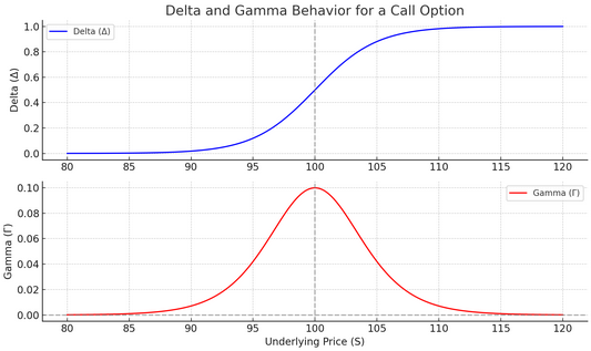
Notice how Delta transitions from ~0 to ~1 as the underlying price rises past the strike price (100). Gamma peaks around the strike price, meaning Delta changes fastest there. As price moves far away from the strike, Gamma fades to near zero. This shows why long positions (+Γ) benefit most when the underlying is near the strike, Delta "accelerates" with movement. Short options (-Γ) are most risky near the strike, since Delta can shift quickly against them.

P&L impact of +Gamma vs. –Gamma:

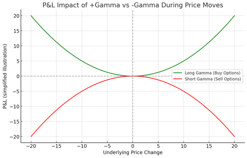
The payoff impact of +Gamma vs -Gamma: profits grow when the market makes large moves (either up or down). This is why long gamma traders want volatility. Losses accelerate when the market makes large moves. Short gamma traders only profit if the market stays calm (low volatility).

Getting Started

//+------------------------------------------------------------------+
//|                                                       G&D222.mq5 |
//|                        GIT under Copyright 2025, MetaQuotes Ltd. |
//|                     https://www.mql5.com/en/users/johnhlomohang/ |
//+------------------------------------------------------------------+
#property copyright "GIT under Copyright 2025, MetaQuotes Ltd."
#property link      "https://www.mql5.com/en/users/johnhlomohang/"
#property version   "1.00"
#property script_show_inputs

#include <Math\Stat\Normal.mqh>
#include <Trade\SymbolInfo.mqh>

To get started, we set up a basic MQL5 script with specific properties and includes essential libraries. The #property script_show_inputs tells MetaTrader 5 to display input parameters in the script’s input dialog when it’s launched. Followed by #include <Math\Stat\Normal.mqh>, which imports statistical functions such as the normal distribution, used for probability and option pricing calculations. Lastly, #include <Trade\SymbolInfo.mqh> provides access to detailed information about the trading symbol (like tick size, point value, or contract size), essential for precise market and instrument handling.

// -------------------- Utility functions ---------------------------
// Standard normal PDF
double NormalPDF(double x)
{
   return MathExp(-0.5*x*x)/MathSqrt(2.0*M_PI);
}

// Standard normal CDF (Abramowitz-Stegun)
double NormalCDF(double x)
{
   double a1= 0.254829592, a2=-0.284496736, a3=1.421413741, a4=-1.453152027, a5=1.061405429, p=0.3275911;
   int sign = 1;
   if(x < 0) { sign = -1; x = -x; }
   double t = 1.0/(1.0 + p*x);
   double y = 1.0 - (((((a5*t + a4)*t) + a3)*t + a2)*t + a1)*t*MathExp(-x*x);
   return 0.5*(1.0 + sign*y);
}

In this section of the code, we define two utility functions to support the mathematical foundation of the Black-Scholes model. The NormalPDF() function computes the probability density function (PDF) of the standard normal distribution, which measures how likely a value is to occur within a continuous probability distribution. It’s a key element in calculating option sensitivities such as delta and gamma, since these rely on the statistical properties of normally distributed returns.

The NormalCDF() function estimates the cumulative distribution function (CDF) of the standard normal distribution using the Abramowitz-Stegun approximation, a well-known numerical method for efficiently computing the area under the normal curve. This function allows the model to determine the probability that a variable will fall below a specific value—a critical step in assessing option price probabilities and risk exposure in financial models.

// Black-Scholes d1,d2
void BS_d1d2(double S, double K, double sigma, double T, double r, double q, double &d1, double &d2)
{
   if(T <= 0 || sigma <= 0) { d1 = d2 = 0.0; return; }
   double sqt = sigma * MathSqrt(T);
   d1 = (MathLog(S/K) + (r - q + 0.5*sigma*sigma)*T) / sqt;
   d2 = d1 - sqt;
}

// Black-Scholes Delta for call
double BS_DeltaCall(double S, double K, double sigma, double T, double r, double q)
{
   if(T <= 0) return (S > K) ? 1.0 : 0.0;
   double d1,d2; BS_d1d2(S,K,sigma,T,r,q,d1,d2);
   return MathExp(-q*T) * NormalCDF(d1);
}

// Black-Scholes Gamma (same for calls and puts)
double BS_Gamma(double S, double K, double sigma, double T, double r, double q)
{
   if(T <= 0 || sigma <= 0) return 0.0;
   double d1,d2; 
   BS_d1d2(S,K,sigma,T,r,q,d1,d2);
   double pdf = NormalPDF(d1);
   return (pdf * MathExp(-q*T)) / (S * sigma * MathSqrt(T));
}

The first function, BS_d1d2(), calculates the intermediate variables d₁ and d₂, which are essential components of the Black-Scholes option pricing model. These terms quantify the standardized distance between the current price and the strike price of an option, adjusted for volatility and time to expiration. Essentially, they help determine the probability of an option finishing in-the-money, forming the mathematical backbone for calculating option sensitivities and prices.

The second function, BS_DeltaCall(), computes the delta of a call option, which measures how much the option’s price is expected to change in response to a small change in the underlying asset’s price. A higher delta means the option behaves more like the underlying asset itself. In this formula, the delta is adjusted by the dividend yield (q), making it more realistic for assets that pay dividends or carry holding costs—a key consideration for stocks like EU50.

Finally, the BS_Gamma() function calculates gamma, the rate of change of delta relative to price movement. Gamma provides insight into the curvature or convexity of the option’s value, indicating how delta will evolve as the market moves. High gamma values suggest that an option’s delta is highly sensitive to price changes, which is crucial information for hedging and risk management strategies like gamma scalping.

// Calculate days until December 31, 2025
double DaysUntilExpiry()
{
   datetime expiry = D'2025.12.31 23:59:59';
   datetime current = TimeCurrent();
   double days = (expiry - current) / (60.0 * 60.0 * 24.0);
   return MathMax(days / 365.0, 0.0); // Convert to years
}

// -------------------- Input parameters ------------------------
input double   K           = 5000.0;    // Strike price (adjust based on current EU50 price)
input double   r           = 0.04;      // Interest rate (4% - more realistic for current rates)
input double   sigma       = 0.1691;    // Annualized volatility (16.91% as specified)
input int      BarsToCalc  = 100;       // How many bars back to calculate
input double   q           = 0.02;      // Dividend yield (2% - typical for EU50)

The function, DaysUntilExpiry(), calculates the remaining time until December 31, 2025, expressed in years. It does so by finding the difference between the current time and the expiry date in seconds, converting that into days, and then dividing by 365. This value represents the time to maturity (T) used in the Black-Scholes model, a key input that affects how option values decay over time (known as theta decay). The use of MathMax() ensures the returned value never goes below zero, even if the current date is past expiry.

The second section defines input parameters that make the script flexible and adaptable to different market conditions. These include the strike price (K), interest rate (r), volatility (sigma), the number of bars to calculate (BarsToCalc), and the dividend yield (q). Together, these inputs allow traders to model realistic market environments—particularly for assets like EU50, where interest rates, volatility, and dividends play a significant role in pricing and risk assessment.

// -------------------- Main calculation function --------------------------------
void OnStart()
{
   Print("Starting Delta and Gamma calculation for ", _Symbol, " with Dec 2025 expiry...");
   
   // Calculate dynamic time to expiry
   double timeToExpiry = DaysUntilExpiry();
   
   PrintFormat("Time to expiry: %.4f years (%.0f days)", timeToExpiry, timeToExpiry * 365);

   // Get historical data
   MqlRates rates[];
   int copied = CopyRates(_Symbol, PERIOD_D1, 0, BarsToCalc, rates);
   
   if(copied <= 0)
   {
      Print("Failed to get historical data. Error: ", GetLastError());
      return;
   }
   
   PrintFormat("Successfully retrieved %d bars of historical data", copied);

   // Create CSV filename with symbol and timestamp
   string filename = "EU50_DeltaGamma_" + IntegerToString(TimeCurrent()) + ".csv";
   int handle = FileOpen(filename, FILE_WRITE|FILE_CSV|FILE_ANSI, ',');
   
   if(handle == INVALID_HANDLE)
   {
      Print("Failed to open file for writing. Error: ", GetLastError());
      return;
   }

   // Write CSV headers
   FileWrite(handle, "Date", "Time", "Close", "Delta", "Gamma", "Strike", "TimeToExpiry_Days");
   
   Print("\n=== EU50 Delta and Gamma Calculations (Dec 2025 Expiry) ===");
   Print("Date\t\tClose\t\tDelta\t\tGamma\t\tDays to Expiry");
   Print("----------------------------------------------------------------");

   int displayCounter = 0;
   // Calculate delta and gamma for each bar (from oldest to newest)
   for(int i = copied - 1; i >= 0; i--)
   {
      // Calculate time to expiry for each historical point
      datetime barTime = rates[i].time;
      datetime expiry = D'2025.12.31 23:59:59';
      double daysToExpiry = (expiry - barTime) / (60.0 * 60.0 * 24.0);
      double T_historical = MathMax(daysToExpiry / 365.0, 0.0);
      
      double S = rates[i].close;
      double delta = BS_DeltaCall(S, K, sigma, T_historical, r, q);
      double gamma = BS_Gamma(S, K, sigma, T_historical, r, q);
      
      // Format date and time
      string dateStr = TimeToString(rates[i].time, TIME_DATE);
      string timeStr = TimeToString(rates[i].time, TIME_MINUTES);
      
      // Write to CSV file
      FileWrite(handle, 
               dateStr,
               timeStr,
               DoubleToString(S, 2),
               DoubleToString(delta, 6),
               DoubleToString(gamma, 6),
               DoubleToString(K, 2),
               DoubleToString(daysToExpiry, 1));
      
      // Print to Experts tab (with formatting for readability)
      if(displayCounter % 15 == 0 || i == copied - 1 || i == 0) // Print every 15th bar plus first and last
      {
         PrintFormat("%s\t%.2f\t%.6f\t%.6f\t%.0f days", 
                    dateStr, S, delta, gamma, daysToExpiry);
      }
      displayCounter++;
   }

   FileClose(handle);
   
   // Calculate current values with exact time to expiry
   double currentT = DaysUntilExpiry();
   double currentPrice = SymbolInfoDouble(_Symbol, SYMBOL_BID);
   double currentDelta = BS_DeltaCall(currentPrice, K, sigma, currentT, r, q);
   double currentGamma = BS_Gamma(currentPrice, K, sigma, currentT, r, q);
   
   Print("");
   Print("==============================================================");
   PrintFormat("CALCULATION COMPLETE - Results saved to: %s", filename);
   Print("");
   Print("CURRENT MARKET VALUES:");
   PrintFormat("EU50 Price: %.2f", currentPrice);
   PrintFormat("Strike: %.2f", K);
   PrintFormat("Moneyness: %.2f%%", (currentPrice/K - 1.0) * 100.0);
   PrintFormat("Delta: %.6f", currentDelta);
   PrintFormat("Gamma: %.6f", currentGamma);
   PrintFormat("Days to Expiry: %.0f", currentT * 365);
   
   Print("");
   Print("PARAMETERS USED:");
   PrintFormat("Volatility: %.4f (16.91%%)", sigma);
   PrintFormat("Interest Rate: %.3f (4%%)", r);
   PrintFormat("Dividend Yield: %.3f (2%%)", q);
   PrintFormat("Total bars processed: %d", copied);
   
   // Risk assessment
   Print("");
   Print("RISK ASSESSMENT:");
   if(currentDelta > 0.7)
      Print("→ High Delta: Option behaves like underlying stock");
   else if(currentDelta > 0.3)
      Print("→ Moderate Delta: Sensitive to price movements");
   else
      Print("→ Low Delta: Limited price sensitivity");
      
   if(currentGamma > 0.02)
      Print("→ High Gamma: Delta changes rapidly with price moves");
   else if(currentGamma > 0.005)
      Print("→ Moderate Gamma: Delta has reasonable sensitivity");
   else
      Print("→ Low Gamma: Delta relatively stable");
   
   Alert("EU50 Delta & Gamma Calculation Complete!\nFile: ", filename,
         "\nCurrent Delta: ", DoubleToString(currentDelta, 4),
         "\nCurrent Gamma: ", DoubleToString(currentGamma, 6));
}

This section defines the main calculation routine (OnStart()) for evaluating Delta and Gamma values of the EU50 index using the Black-Scholes model. The function begins by announcing the start of the calculation and determining the dynamic time to expiry until December 31, 2025. This ensures the computation reflects the remaining time until the option’s maturity, a crucial factor influencing both Delta and Gamma. By printing out the number of years and days left to expiry, the trader gains immediate insight into how close the option is to expiration—a key aspect of time decay risk.

Next, the script retrieves historical daily price data using the CopyRates() function, which fills an array with closing prices for the number of bars specified by the BarsToCalc input. This step is essential for performing a historical analysis of how Delta and Gamma evolved. If the data retrieval fails, the function exits gracefully with an error message, ensuring robustness in real-market testing. Upon successful data acquisition, the script creates a CSV file named dynamically with the current timestamp, allowing for organized storage and easy export for external analysis, such as in Excel or Jupyter Lab.

The code then enters a loop that iterates through historical bars (from oldest to newest), calculating the Delta and Gamma for each closing price. For each bar, the script recalculates time to expiry to reflect how far each data point was from December 31, 2025. The computed values—Delta, Gamma, strike, and days to expiry—are written into the CSV file and printed to the terminal periodically for readability. This design provides traders with a structured dataset that can later be used for visualization and further analysis, such as studying option sensitivity over different market phases.

After processing all bars, the file is closed, and the script computes current market Delta and Gamma values based on the latest price and the exact time remaining until expiry. These current values help the trader understand the real-time exposure of their option position. The script also calculates and prints additional details, such as moneyness, volatility, interest rate, and dividend yield—parameters that collectively define the option’s market environment. This provides a comprehensive summary of both historical and current risk conditions in one view.

Finally, the script includes a risk assessment section, which interprets Delta and Gamma magnitudes qualitatively. High Delta indicates the option behaves similarly to the underlying asset, while low Delta signals less price sensitivity. Similarly, high Gamma suggests that Delta changes rapidly as the underlying price moves—implying higher convexity and potential hedging costs. The function concludes by alerting the user through an on-screen notification, confirming successful completion of calculations, and providing key results for immediate interpretation.

Report Results

Based on the EU50 Delta and Gamma analysis, the results reveal a consistently in-the-money call option position with strong bullish characteristics. The Delta values range from 0.74 to 0.99 throughout the historical period, indicating the option has maintained a high probability of expiring profitably. Currently sitting at 0.991 with 69 days to expiry, the option behaves almost identically to owning the underlying EU50 index, with price movements translating nearly 1:1 to option value changes. The Gamma values, ranging from 0.000186 to 0.000624, demonstrate moderate sensitivity to price changes, with the highest Gamma concentrations occurring when prices dipped closer to the 5,000 strike in late July and early August 2025. This pattern suggests the option was most sensitive to underlying price movements during periods of lower moneyness, particularly when EU50 traded between 5,180 to 5,260.

The temporal analysis shows a clear relationship between time decay and Greek sensitivity. As the option approaches its December 2025 expiry, both Delta and Gamma have become more stable, with Delta converging toward 1.0 and Gamma declining to current levels of 0.000186. The risk assessment indicates this is a low-Gamma, high-Delta position that requires minimal dynamic hedging and behaves predominantly like a long stock position. For traders, this represents a relatively low-maintenance position with limited Gamma risk, though the high Delta means the position carries substantial directional exposure to EU50 price movements. The consistent moneyness throughout the period suggests the strike selection was appropriate for a bullish outlook, providing strong intrinsic value while maintaining reasonable sensitivity characteristics until expiration.

Conclusion

In summary, we developed a complete framework to calculate Black-Scholes Greeks—Gamma and Delta—for real financial instruments like EU50. Starting from the mathematical foundation, we implemented core formulas for Delta, Gamma, and time-to-expiry calculations directly in MQL5, enabling real-time option sensitivity tracking within MetaTrader. We then exported historical data to CSV and performed advanced visualization in Jupyter Lab, examining how Delta and Gamma evolve with price and volatility. The resulting plots—Delta vs. Price, Gamma curvature, and Gamma Exposure (GEX)—provided a clear view of how these sensitivities behave across different market conditions.

In conclusion, this integration of quantitative modeling can empower traders to better understand their option exposure and risk profile. By observing how Gamma amplifies Delta changes near the strike and how GEX reflects potential market stability or volatility, traders can make more informed hedging and entry decisions. This approach bridges the gap between theory and execution, transforming the Black-Scholes Greeks into practical trading insights for dynamic risk management and data-driven strategy refinement.