Reimagining Classic Strategies (Part VII) : Forex Markets And Sovereign Debt Analysis on the USDJPY

Artificial Intelligence holds the potential to create new trading strategies for the modern investor. It is unlikely that any single investor will have enough time to carefully assess each possible strategy before deciding which one to trust with their capital. In this series of articles, we aim to present you with the information you need to arrive at an informed decision as to which strategy best fits your particular investor profile.

Synopsis of The Trading Strategy

Fixed income securities are investments that allow investors to diversify their portfolios safely. They are a class of investments that pay a fixed or floating rate of return until maturity. Upon maturity, the investor’s principal is paid back, and no further payments will be made to the investor. There are many different types of fixed income securities, such as bonds and Certificates of Deposit.

Bonds are among the most popular forms of fixed income securities and will be the focus of our discussion. Bonds may be issued by a Corporation or a Government. Government Bonds in particular are among the safest investments in the World. If an investor wishes to purchase a particular Government’s Bond, they must do so in the Currency of the issuing state. If a particular Government’s Bond is in high demand internationally, every investor desiring to acquire the bond will first convert their domestic Currency into the desired Currency. This may in turn shift the market’s beliefs about a fair valuation of the two currencies' exchange rate. 

How well a bond is performing is measured by the yield of the bond. There is an inverse relationship between the yield of a bond and the level of demand for that bond. In other words, as demand for a particular bond falls, the yield of the bond rises to rally demand for the bond. Some successful traders in the Currency markets incorporate this fundamental analysis into their trading strategy. By comparing the yields of mid-long term Government bonds from the 2 countries in any exchange rate, Currency traders may gain an intuition about the economic conditions of the two countries in question.

Typically, the bond offering investors higher interest rates will be more popular and according to the strategy, the Currency of the issuing country will also appreciate over time, and the Currency of the country issuing bonds with lower interest rates will depreciate over time. 

Synopsis of The Methodology

To assess the strategy, we train various models to predict the closing price of the USDJPY exchange rate. We had 3 sets of predictors for the models:

1. Ordinary Open, High, Low, Close, Tick Volume (OHLCV) data fetched from the USDJPY Market.
2. OHLCV data on the Japanese Government 10-Year Bond and the American Government 10-Year Treasury Note.
3. A super set of the first two.

Our goal was to identify which set of predictors would produce a model with the lowest RMSE on unseen data. Although the correlation levels between the bonds' historical prices and the USDJPY were significantly strong, -0.85 for both Government bonds, the lowest test error rate was produced by models trained from the first set of predictors.

The best model we identified was the Linear Regression (LR) model. However, it has no parameters we can tune. Therefore, we selected the Linear Support Vector Regressor (LSVR) as our candidate solution. We successfully performed hyperparameter tuning on the LSVR model without overfitting to the training set. Furthermore, our customized LSVR model was able to outperform the benchmark performance set by the simpler LR model on validation data. The models were trained and compared using time series cross validation without random shuffling.

After successfully tuning our model, we exported it to ONNX format and integrated it into our customized Expert Advisor. 

Fetching Data

Let us get started, first we shall import the libraries we need.

#Import the libraries we need
import pandas as pd
import numpy as np
import MetaTrader5 as mt5
import matplotlib.pyplot as plt
import matplotlib
import seaborn as sns
import sklearn
from sklearn.preprocessing import RobustScaler
from sklearn.model_selection import train_test_split

Here are the versions of the libraries we are using.

#Show library versions
print(f"Pandas version: {pd.__version__}")
print(f"Numpy version: {np.__version__}")
print(f"MetaTrader 5 version: {mt5.__version__}")
print(f"Matplotlib version: {matplotlib.__version__}")
print(f"Seaborn version: {sns.__version__}")
print(f"Scikit-learn version: {sklearn.__version__}")

Pandas version: 1.5.3

Numpy version: 1.24.4

MetaTrader 5 version: 5.0.45

Matplotlib version: 3.7.1

Seaborn version: 0.13.0

Scikit-learn version: 1.2.2

Let us initialize our terminal.

#Initialize the terminal
mt5.initialize()

True

Defining how far into the future we wish to forecast.

#Define how far ahead into the future we should forecast
look_ahead = 20

Fetching the time-series data that we need from the MetaTrader 5 terminal.

#Fetch historical market data 
usa_10y_bond = pd.DataFrame(mt5.copy_rates_from_pos("UST10Y_U4",mt5.TIMEFRAME_M1,0,100000))
jpn_10y_bond = pd.DataFrame(mt5.copy_rates_from_pos("JGB10Y_U4",mt5.TIMEFRAME_M1,0,100000))
usd_jpy      = pd.DataFrame(mt5.copy_rates_from_pos("USDJPY",mt5.TIMEFRAME_M1,0,100000))

The data frame time column needs to be formatted.

#Convert the time from seconds
usa_10y_bond["time"] = pd.to_datetime(usa_10y_bond["time"],unit="s")
jpn_10y_bond["time"] = pd.to_datetime(jpn_10y_bond["time"],unit="s")
usd_jpy["time"] = pd.to_datetime(usd_jpy["time"],unit="s")

We should set the time column as our index, this will make it easier for us to merge our 3 data frames into 1.

#Prepare to merge the data
usa_10y_bond.set_index("time",inplace=True)
jpn_10y_bond.set_index("time",inplace=True)
usd_jpy.set_index("time",inplace=True)

Merging the data frames.

#Merge the data
merged_data = usa_10y_bond.merge(jpn_10y_bond,how="inner",left_index=True,right_index=True,suffixes=(" usa"," japan"))
merged_data = merged_data.merge(usd_jpy,left_index=True,right_index=True)

Exploratory Data Analysis

Let us create a copy of the data frame that we will use for plotting purposes.

data_visualization = merged_data

We need to reset the index of the visualization data.

#Reset the index
data_visualization.reset_index(inplace=True)

Scale all the column values so that they all begin with one.

#Let's scale the data so all the first values in the column are one
for i in np.arange(1,data_visualization.shape[1]):
    data_visualization.iloc[:,i] = data_visualization.iloc[:,i] / data_visualization.iloc[0,i]

Let us plot the 3 time-series to see if there are any observable relationships.

#Let's create a plot
plt.figure(figsize=(10, 5))
plt.plot(data_visualization.loc[:,"open usa"])
plt.plot(data_visualization.loc[:,"open japan"])
plt.plot(data_visualization.loc[:,"open"])
plt.legend(["USA 10Y T-Note","JGB 10Y Bond","USDJPY Fx Rate"])

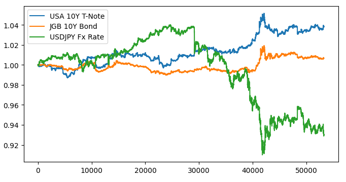
Fig 1: Visualizing our market data.

There appears to be no discernible relationship when we overlay the 3 markets. Let us try and make the plot easier to read, by plotting the spread between the American and Japanese bonds. That way, we only need to consider the USDJPY exchange rate and the USA JPY 10-Y Bond spread. Or in other words, the 3 curves we plotted above, can be fully represented by only 2 curves.

First, we need to calculate the spread between the bonds.

#Let's create a new feature to show the spread between the securities
data_visualization["spread"] = data_visualization["open usa"] - data_visualization["open japan"]

On the left side of the chart, we see a sample of the USDJPY exchange rate, whenever the exchange rate surpasses 1, the Dollar is performing better than the Yen, the opposite holds true when the exchange rate falls below 1. Furthermore, whenever the spread rises above 0, the American bonds are performing better than the Japanese bonds and the converse is true when the spread falls below 0. Therefore, when the spread is below 0 meaning the Japanese bonds are performing better in the market, we would also expect to see the equilibrium exchange shift in favor of the Yen. However, by visually inspecting the plots with our eyes, we can quickly observe that this expectation does not always hold true.

#Visualizing the results of using the bonds predictors
fig,axs = plt.subplots(1,2,sharex=True,sharey=False,figsize=(8,4))
columns = ["open","spread"]

for i,ax in enumerate(axs.flat):
    ax.plot(data_visualization.loc[:,columns[i]])
    ax.set_title(columns[i])

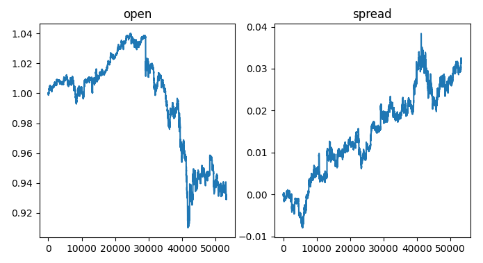
Fig 2: Visualizing the bond spread on the exchange rate.

Let us now label our data. 

#Label the data
merged_data["target"] = merged_data["close"].shift(-look_ahead)
merged_data["binary target"] = np.nan
merged_data.loc[merged_data["close"] > merged_data["target"],"binary target"] = 0
merged_data.loc[merged_data["close"] < merged_data["target"],"binary target"] = 1
merged_data.dropna(inplace=True)
merged_data.reset_index(inplace=True)
merged_data

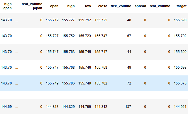
Fig 3: The current state of our data frame.

Now we need to define our target and inputs.

#Define the predictors and target
target = "target"
ohlc_predictors = ['open', 'high', 'low', 'close','tick_volume']
bonds_predictors = ['open usa','high usa','low usa','close usa','tick_volume usa','open japan','high japan', 'low japan', 'close japan','tick_volume japan']
predictors = ['open usa','high usa','low usa','close usa','tick_volume usa','open japan','high japan', 'low japan', 'close japan','tick_volume japan','open', 'high', 'low', 'close','tick_volume']

Let us analyze the correlation levels in our dataset.

#Analyze correlation levels
plt.subplots(figsize=(8,6))
sns.heatmap(merged_data.loc[:,predictors].corr(),annot=True)

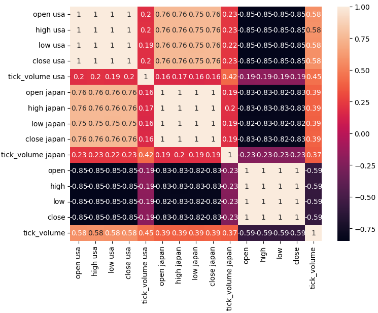
Fig 4: Our correlation matrix.

As we can observe, there are strong correlation levels between the American and Japanese bonds, 0.76. Furthermore, both the American and Japanese bond securities have strong negative correlation levels with the USDJPY exchange rate. 

Scatter plots allow us to visualize relationships between variables in 2 dimensions, let us create scatter plots using the data we have collected from the bond market. We will start by creating a scatter plot of the opening price of the American Treasury note against the opening price of the USDJPY exchange rate.

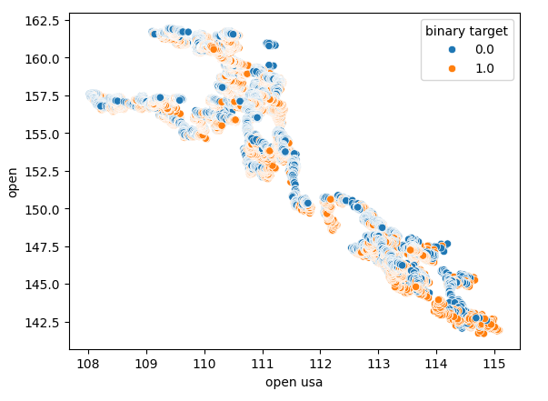
Fig 5: A scatter plot of the USA Bond Open price against the USDJPY Open price.

As one can observe, there is no clear pattern or dependency being exposed by the scatter plot. It appears that the exchange rate may appreciate or depreciate, regardless of the changes occurring in the bond market.

We also performed another scatter plot using the opening price of the Japanese Government bond on the x-axis and the opening price of the USDJPY exchange rate on the y-axis. Unfortunately, there was still no visible relationship in the data.

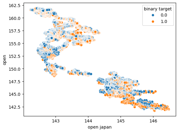
Fig 6: A scatter plot of the Japanese Government Bond Open price against the USDJPY Open price.

We also tried to create another scatter plot, this time using both Government bonds on each axis. We used the opening price of the Japanese Government bond on the x-axis, and the American Treasury notes were on the y-axis. Our scatter plot didn’t reveal any interesting patterns in the data, this may indicate to us that there may be other variables we aren’t considering that are also affecting the data.

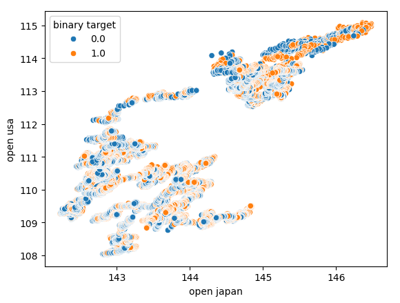
Fig 7: A scatter plot of the Japanese Government Bond Open price against the American Government Bond Open price.

Let us also check to see if there is any relationship between the tick volume of the American bond market and the closing price of the USDJPY exchange rate. Unfortunately, there is no clear separation in the scatter plot, we observe many instances where price rose and fell on the same tick volume reading.

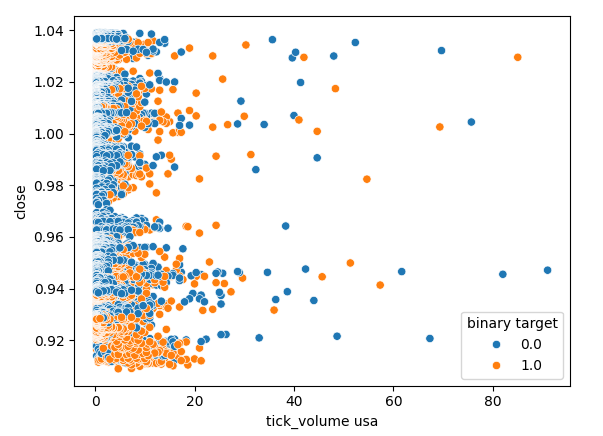
Fig 8: A scatter plot of the American Government Bond tick volume against the USDJPY Close price.

Modelling The Data

We are now ready to start modelling our data, we will start off by scaling and standardizing our dataset. This helps our machine learning models learn effectively.

#Scale the data
scaled_data = pd.DataFrame(RobustScaler().fit_transform(merged_data.loc[:,predictors]),columns=predictors)

Then we will partition our dataset into two halves, one half will be used to train and optimize our models, while the latter will be used to validate our models and test for overfitting.

#Partition the data
train_X , test_X, train_y, test_y = train_test_split(scaled_data,merged_data.loc[:,target],shuffle=False,test_size=0.5)

To effectively test various models, we will keep our models in a list so that we can loop over them and cross validate each of their performances in turn. We will also need to create 3 data frames:

1. The first data frame will store our error levels when only using ordinary OHLCV data from the USDJPY market.
2. The second data frame will store our error levels when only relying on OHCLV data from both bond markets.
3. And the last data frame will store our error levels when incorporating all the data we have available.

#Model selection
from sklearn.linear_model import LinearRegression , Lasso , SGDRegressor
from sklearn.svm import LinearSVR
from sklearn.ensemble import GradientBoostingRegressor , RandomForestRegressor , BaggingRegressor
from sklearn.neighbors import KNeighborsRegressor
from sklearn.neural_network import MLPRegressor
from sklearn.metrics import mean_squared_error 
from sklearn.model_selection import TimeSeriesSplit

#Define the columns
columns = [
    "Linear Model",
    "Lasso",
    "SGD",
    "Linear SV",
    "Gradient Boost",
    "Random Forest",
    "Bagging",
    "K Neighbors",
    "Neural Network"
]

#Define the models
models = [
    LinearRegression(),
    Lasso(),
    SGDRegressor(),
    LinearSVR(),
    GradientBoostingRegressor(),
    RandomForestRegressor(),
    BaggingRegressor(),
    KNeighborsRegressor(),
    MLPRegressor(hidden_layer_sizes=(100,40,20,10),shuffle=False)
]

#Create 2 dataframes to store our error on the training and test sets respectively
ohlc_training_loss = pd.DataFrame(index=np.arange(0,5),columns=columns)
ohlc_validation_loss = pd.DataFrame(index=np.arange(0,5),columns=columns)
bonds_training_loss = pd.DataFrame(index=np.arange(0,5),columns=columns)
bonds_validation_loss = pd.DataFrame(index=np.arange(0,5),columns=columns)
all_training_loss = pd.DataFrame(index=np.arange(0,5),columns=columns)
all_validation_loss = pd.DataFrame(index=np.arange(0,5),columns=columns)
#Create the time-series split object
tscv = TimeSeriesSplit(n_splits=5,gap=look_ahead)

We will now cross validate each of our models. The outer loop will iterate over each model we have available, while the inner loop will cross validate each model and store our respective training and test error levels. Note that we are cross validating the models on the training set only.

#Now perform cross validation
for j in np.arange(0,len(models)):
    model = models[j]
    for i,(train,test) in enumerate(tscv.split(train_X)):
        model.fit(train_X.loc[train[0]:train[-1],predictors],train_y.loc[train[0]:train[-1]])
        all_training_loss.iloc[i,j] = mean_squared_error(train_y.loc[train[0]:train[-1]],model.predict(train_X.loc[train[0]:train[-1],predictors]))
        all_validation_loss.iloc[i,j] = mean_squared_error(train_y.loc[test[0]:test[-1]],model.predict(train_X.loc[test[0]:test[-1],predictors]))

Let us now observe our error levels when using ordinary OHLCV data from the USDJPY market. As we can see, the linear model performed and the Linear Support Vector regressor performed notably well in this particular setup.

#Our results using the OHLC data
ohlc_validation_loss

Fig 9: Our OHLCV error levels.

Let us visualize the results. We will start off with a line plot of the performance of each model in our 5-fold cross validation procedure.

#Visualizing the results of using the OHLC predictors
plt.plot(ohlc_validation_loss)
plt.legend(columns)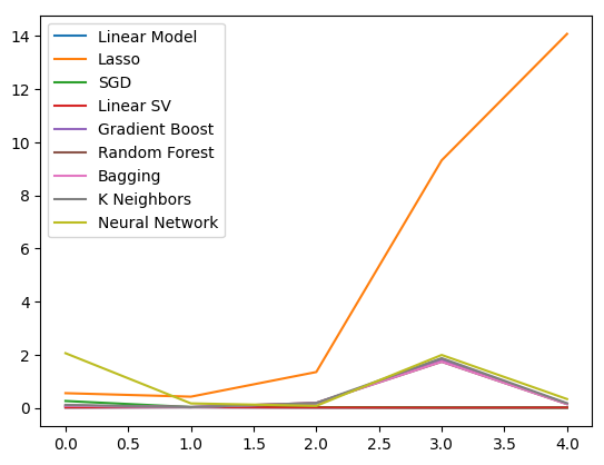

Fig 10: Line plots of our OHLCV error values. 

We can clearly see that the Lasso was the worst performing model, its validation error rate was the greatest by a significant margin. However, it is not clear which model is achieving the lowest error rate, we can use box plots to answer that question.

Box plots help us quickly identify which models are performing well in this particular task. As we can see from the plot below, the linear regression has the lowest average error levels, furthermore it appears stable and it has the lowest outlier value.

#Visualizing the results of using the OHLC predictors
fig,axs = plt.subplots(2,4,sharex=True,sharey=True,figsize=(16,10))

for i,ax in enumerate(axs.flat):
    ax.boxplot(ohlc_validation_loss.iloc[:,i])
    ax.set_title(columns[i])

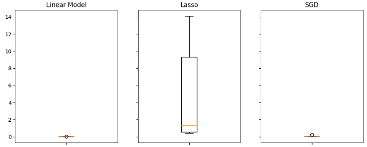
Fig 11: Some of our error levels when using ordinary USDJP OHLCV

When we used the data related to the government bonds, our performance levels dropped across the board. However, the Linear Support Vector Regressor (Linear SVR) appears to be able to handle this data quite well.

#Our results using the bonds data
bonds_validation_loss

Fig 12: Our error levels when using the bonds data.

Let us visualize the results.

#Visualizing the results of using the bonds predictors
plt.plot(bonds_validation_loss)
plt.legend(columns)

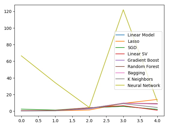
Fig 13: A line plot of our validation error when using Bond Data to predict the USDJPY exchange rate.

We can also employ box plots to assess our error levels.

#Visualizing the results of using the bonds predictors
fig,axs = plt.subplots(2,4,sharex=True,sharey=True,figsize=(16,10))

for i,ax in enumerate(axs.flat):
    ax.boxplot(bonds_validation_loss.iloc[:,i])
    ax.set_title(columns[i])

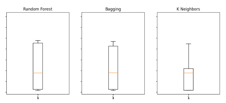
Fig 14: Some of our error levels when using OHLCV data from the Bond market to predict the future close price of the USDJPY

Finally, when we incorporated all the available data, our error levels improved in comparison to our previous step, however they were not as satisfactory when compared to our error levels using just the market quotes from the USDJPY market.

#Our results using all the data we have
all_validation_loss

Fig 15: Our error levels when using all the data we have.

Let us visualize our performance.

#Visualizing the results of using the bonds predictors
plt.plot(all_validation_loss)
plt.legend(columns)

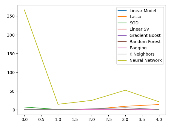
Fig 16:Our error levels when predicting the USDJPY close using all the data we have.

The Linear Regression model is clearly our best option here. However, it no hyperparameters of interest to us. Therefore, we will select the second-best model, the Linear SVR, and attempt to tune it to outperform the Linear model without overfitting to the training set. Before optimizing the model, let us assess which features are important to the model. If our strategy is viable, we would expect our feature elimination algorithms to retain the column. Otherwise, if the bond data is discarded we may have reason to revise the strategy.

#Visualizing the results of using the bonds predictors
fig,axs = plt.subplots(2,4,sharex=True,sharey=True,figsize=(16,10))

for i,ax in enumerate(axs.flat):
    ax.boxplot(all_validation_loss.iloc[:,i])
    ax.set_title(columns[i])

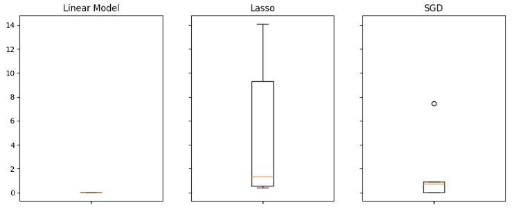
Fig 17: Our Linear Model performed the best when using all the available data.

Feature Selection

Let us first start by calculating Shapley (SHAP) values. SHAP values are a metric designed to inform us the impact that each input has on our model’s predictions, when compared to a baseline value for each column. For example, consider a model predicting the likelihood of a driver getting a speeding ticket. If we wanted to assess whether our model is capable of making reasonable predictions, we may ask, “How does our model interpret the fact that the driver’s blood alcohol level is high?”.

Obviously, we would expect our model to predict higher probabilities of getting a speeding ticket if you’re driving under the influence of alcohol. SHAP Values help us answer questions of this nature by rephrasing the question to include a baseline value, “How does our model interpret the fact that the driver’s blood alcohol level is above the legal limit?”.

By including the legal limit, we have defined a baseline. Therefore, we calculate our SHAP Values by performing calculations on the difference between the model’s predictions when the driver’s blood alcohol levels are beneath and above the legal limits. 

Let us import the SHAP library.

#Feature selection
import shap

Now, we need to train our model.

#The SVR performed quite well, let's inspect it further
model = LinearSVR()
model.fit(train_X,train_y)

Let us fit the SHAP explainer.

#Calculate SHAP Values
explainer = shap.Explainer(model.predict,test_X)
shap_values = explainer(test_X)

Let us view the SHAP plot.

shap.plots.beeswarm(shap_values)

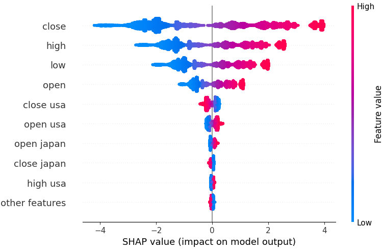
Fig 18: Our SHAP Values from our Linear SVR model.

The features are arranged in order, starting with the most important at the top. Therefore, it appears that the close value of the USDJPY is the most important feature according to our SHAP explanations. Furthermore, we can also see that our data related to the government bonds was just after all the price data of the Currency pair. This is good evidence backing our strategy, our SHAP values consider that the bond data is more important than the tick volume of the USDJPY market itself.

However, all model explanations must be taken with a grain of salt. They are not immune to error.

Let us also consider backward selection. The backward selection algorithm begins by fitting a full model, and eliminates features sequentially until the test error can no longer by improved. 

Let us import the mlxtend library.

#Let's also perform backward selection
from mlxtend.feature_selection import SequentialFeatureSelector as SFS
from mlxtend.plotting import plot_sequential_feature_selection as plot_sfs

Initialize the model.

#Reinitialize the model
model = LinearSVR()

Create the feature selector object.

#Prepare the feature selector
sfs = SFS(model,
         k_features=(1,train_X.shape[1]),
         forward=False,
          n_jobs = -1,
          scoring="neg_mean_squared_error",
          cv=5)

Fit the feature selector.

#Fit the feature selector
sfs_results = sfs.fit(train_X,train_y)

Let us see the features selected.

#The best features we identified
sfs_results.k_feature_names_

('open usa',

 'high usa',

 'tick_volume usa',

 'open japan',

 'low japan',

 'close',

 'tick_volume')

Our backward elimination algorithm gave more importance to the bond market data than our SHAP Values. Therefore, we may reasonably conclude that there may be a reliable relationship between our bond data and the future exchange rate of the USDJPY pair.

Let us plot the results.

#Prepare the plot
fig1 = plot_sfs(sfs_results.get_metric_dict(),kind="std_dev")
plt.title("Backward Selection on our Linear SVR")
plt.grid()

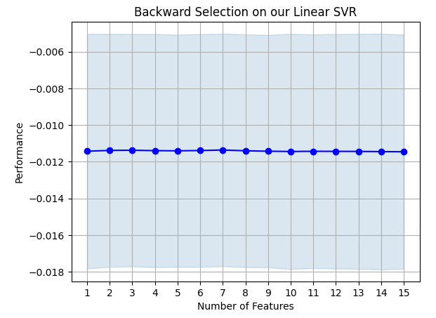
Fig 19: Our backward elimination results.

It appears that our model's error rates do not violently fluctuates, meaning that our model may be stable even under circumstances of limited data. Remember, the algorithm eliminates features one by one until the error rate cannot be improved anymore by removing any of the features selected by the algorithm.

Hyperparameter Tuning

Let us now optimize our model to outperform the Linear Regression.

First, import the libraries we need.

#Parameter tuning 
from sklearn.model_selection import RandomizedSearchCV

Initialize the model.

#Reinitialize the model
model = LinearSVR()

Define the tuner object.

tuner = RandomizedSearchCV(model,
                          {
                              "epsilon":[0,0.001,0.01,0.1,25,50,100],
                              "tol": [0.1,0.01,0.001,0.0001,0.00001],
                              "C" : [1,5,10,50,100,1000,10000,100000],
                              "loss":["epsilon_insensitive", "squared_epsilon_insensitive"],
                              "fit_intercept": [False,True]
                          },
                           n_jobs=-1,
                           n_iter=100,
                           scoring="neg_mean_squared_error"
                          )

Tune the model.

tuner_results = tuner.fit(train_X,train_y)

It’s quite interesting to note that our best parameters are almost identical to the default settings. However, let us observe the difference in performance.

tuner_results.best_params_

{'tol': 0.0001,

 'loss': 'epsilon_insensitive',

 'fit_intercept': True,

 'epsilon': 0,

 'C': 1}

Testing For Overfitting

Let us now test if we were overfitting the training set. We will instantiate our models.

#Testing for overfitting
baseline_model = LinearRegression()
default_model =  LinearSVR()
customized_model = LinearSVR(tol=0.0001,loss='epsilon_insensitive',fit_intercept=True,epsilon=0,C=1)

Now, let us fit all 3 models.

#Fit the models
baseline_model.fit(train_X,train_y)
default_model.fit(train_X,train_y)
customized_model.fit(train_X,train_y)

Preparing to cross validate each model’s performance.

#Create a list of models
models = [
    baseline_model,
    default_model,
    customized_model
]

columns = [
    "Linear Regression",
    "Default Linear SVR",
    "Customized Linear SVR"
]

We need to reset the index of our datasets.
#Let's assess our new accuracy levels
test_y = test_y.reset_index()
test_X.reset_index(inplace=True)

Redefine the time series split object and create a data frame to store our validation error.

#Create our time-series test object
tscv = TimeSeriesSplit(n_splits=5,gap=look_ahead)
overfitting_error = pd.DataFrame(columns=columns,index=np.arange(0,5))

Cross-validate each model.
for j in np.arange(0,len(columns)):
    model = models[j]
    for i , (train,test) in enumerate(tscv.split(test_X)):
        model.fit(test_X.loc[train[0]:train[-1],predictors],test_y.loc[train[0]:train[-1],"target"])
        overfitting_error.iloc[i,j] = mean_squared_error(test_y.loc[test[0]:test[-1],"target"],model.predict(test_X.loc[test[0]:test[-1],predictors]))

Let us see the results.

#Visualizing the results of using the bonds predictors
fig,axs = plt.subplots(1,3,sharex=True,sharey=True,figsize=(8,4))

for i,ax in enumerate(axs.flat):
    ax.boxplot(overfitting_error.iloc[:,i])
    ax.set_title(columns[i])

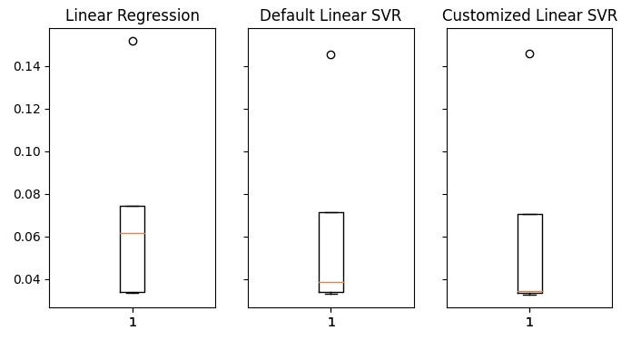
Fig 20: Our error levels on unseen data

We can clearly see that our LinearSVR model produced the lowest average error in validation. Therefore, we have managed to outperform the benchmark set by the Linear Model. Furthermore, we also outperformed the default error rate without overfitting to the training set.

Exporting To ONNX

Let us now prepare to export our model to ONNX format so that we can easily integrate it into our MQL5 program.

Before we can progress, we must first standardize our data in a fashion we can reproduce in MQL5. We can accomplish this by subtracting the column mean from each respective column value, and subsequently dividing each column by its standard deviation.

Let us write out the respective values to a CSV file, in our Terminal’s file path.

#Create scaling factors
scaling_factors = pd.DataFrame(index=("mean","standard deviation"),columns=predictors)

#Write our the values
for i in np.arange(0,scaling_factors.shape[1]):
    scaling_factors.iloc[0,i] = merged_data.loc[:,predictors[i]].mean()
    scaling_factors.iloc[1,i] = merged_data.loc[:,predictors[i]].std()
    merged_data.loc[:,predictors[i]] = ((merged_data.loc[:,predictors[i]] - scaling_factors.iloc[0,i]) / scaling_factors.iloc[1,i])

scaling_factors

Fig 21: Our scaling factors.

Now we shall save the CSV file.

#Save the scaling factors
scaling_factors.to_csv("C:\\Enter \\Your\\Path\\Here\\MetaQuotes\\Terminal\\D0E82094358C8CF3394F550E51FF075\\MQL5\\Files\\usdjpy scaling factors.csv")

Let us train the model on all the data we have available.

#Fit the model on all the data we have
customized_model.fit(merged_data.loc[:,predictors],merged_data.loc[:,"target"])

Import the libraries we need.

#Let's import the libraries we need
from skl2onnx.common.data_types import FloatTensorType
from skl2onnx import convert_sklearn
import netron
import onnx

Define the input type and shape of our ONNX model.

#Define the initial input types
initial_types = [('float_input',FloatTensorType([1,len(predictors)]))]

Create an ONNX model.

#Create an ONNX representation of the model
onnx_model = convert_sklearn(customized_model,initial_types=initial_types,target_opset=12)

Save the ONNX model to a file with the .onnx extension.

#Save the ONNX model
onnx_name = "USDJPY M1 FLOAT.onnx"
onnx.save(onnx_model,onnx_name)

Let us visualize the model in netron.

#Visualize the model
netron.start(onnx_name)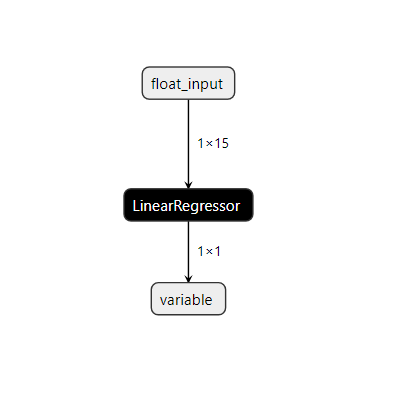

Fig 22: Visualizing our Linear SVR model.

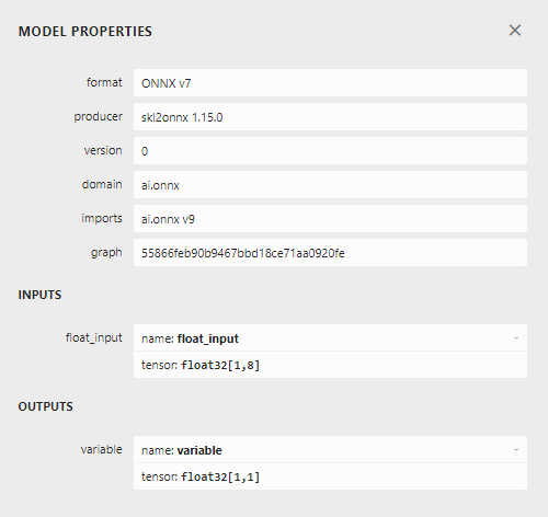
Fig 23: Our ONNX model input and output shape.

Our model’s input and output shape are inline with our specifications. Let us proceed to build the Expert Advisor.

Implementation in MQL5

We shall first require our ONNX model as a resource that will be compiled into our program.

//+------------------------------------------------------------------+
//|                                                 USDJPY Bonds.mq5 |
//|                                               Gamuchirai Ndawana |
//|                    https://www.mql5.com/en/users/gamuchiraindawa |
//+------------------------------------------------------------------+
#property copyright "Gamuchirai Ndawana"
#property link      "https://www.mql5.com/en/users/gamuchiraindawa"
#property version   "1.00"

//+------------------------------------------------------------------+
//| Resources                                                        |
//+------------------------------------------------------------------+
#resource "\\Files\\USDJPY M1 FLOAT.onnx" as const uchar onnx_model_buffer[];

Now let us define a few global variables we need throughout our program.

//+------------------------------------------------------------------+
//| Global variables                                                 |
//+------------------------------------------------------------------+
long onnx_model;
float mean_values[15],std_values[15];
vector model_output = vector::Zeros(1);
int state = 0;
int prediction = 0;

Import the trade library so we can easily open and manage positions.

//+------------------------------------------------------------------+
//| Libraries                                                        |
//+------------------------------------------------------------------+
#include <Trade/Trade.mqh>
CTrade Trade;

Now we shall define helper functions for our Expert Advisor. We need a function that will load our ONNX model and define its input and output shapes. If we fail at any point in the procedure, our function will return a flag that will break the initialization procedure.

//+------------------------------------------------------------------+
//| Load our onnx file                                               |
//+------------------------------------------------------------------+
bool load_onnx_file(void)
  {
//--- Create the model from the buffer
   onnx_model = OnnxCreateFromBuffer(onnx_model_buffer,ONNX_DEFAULT);

//--- Set the input shape
   ulong input_shape [] = {1,15};

//--- Check if the input shape is valid
   if(!OnnxSetInputShape(onnx_model,0,input_shape))
     {
      Alert("Incorrect input shape, model has input shape ", OnnxGetInputCount(onnx_model));
      return(false);
     }

//--- Set the output shape
   ulong output_shape [] = {1,1};

//--- Check if the output shape is valid
   if(!OnnxSetOutputShape(onnx_model,0,output_shape))
     {
      Alert("Incorrect output shape, model has output shape ", OnnxGetOutputCount(onnx_model));
      return(false);
     }
//--- Everything went fine
   return(true);
  }

We also need a function to read the CSV file that has the scaling values and store them in an array for us to use later, in our predict function. Note that, the first row only contains the column titles. The first entry in the second row is the index label, and the second entry in the second row is the mean of the first column. Therefore, our function will check the current loop iteration to keep track of where it is and which values are important.

//+------------------------------------------------------------------+
//| Load our scaling factors                                         |
//+------------------------------------------------------------------+
void load_scaling_factors(void)
    {
//--- Read in the file
   string file_name = "usdjpy scaling factors.csv";

//--- Try open the file
   int result = FileOpen(file_name,FILE_READ|FILE_CSV|FILE_ANSI,","); //Strings of ANSI type (one byte symbols). 

//--- Check the result
   if(result != INVALID_HANDLE)
     {
      Print("Opened the file");
      //--- Store the values of the file
      
      int counter = 0;
      string value = "";
      
      while(!FileIsEnding(result) && !IsStopped()) //read the entire csv file to the end 
       {
       
         if (counter > 100) //if you aim to read 10 values set a break point after 10 elements have been read
           break; //stop the reading progress
         
         value = FileReadString(result);
         Print("Trying to read string: ",value," count value: ",counter);
         
         //--- Check where we are
         if((counter >= 17) && (counter < 32))
            {
               mean_values[counter - 17] = (float) value;
            }   
         //--- Check where we are
         if((counter >= 33) && (counter < 48))
            {
               std_values[counter - 33] = (float) value;
            }   
         //--- Reading a new row
         if(FileIsLineEnding(result))
           { 
             Print("row++");
           }
         
         counter++;
       }
      //---Close the file
      ArrayPrint(mean_values);
      ArrayPrint(std_values);
      FileClose(result);
     }
//--- We failed to find the file
else 
   {
      Print("Failed to find the file");
   }

  }

This function will fetch our model input values and standardize them before obtaining a prediction from our model. Subsequently, the model’s prediction will be stored as a binary state, 1 is a bullish prediction and 2 is a bearish position. This will help us identify when our model is predicting a reversal.

//+------------------------------------------------------------------+
//| Obtain a prediction from our model                               |
//+------------------------------------------------------------------+
void model_predict(void)
   {
     //--- Fetch input values
      string symbols[3] = {"UST10Y_U4","JGB10Y_U4","USDJPY"};
      vectorf model_inputs = {iOpen(symbols[0],PERIOD_CURRENT,0),iHigh(symbols[0],PERIOD_CURRENT,0),iLow(symbols[0],PERIOD_CURRENT,0),iClose(symbols[0],PERIOD_CURRENT,0),iTickVolume(symbols[0],PERIOD_CURRENT,0),
                      iOpen(symbols[1],PERIOD_CURRENT,0),iHigh(symbols[1],PERIOD_CURRENT,0),iLow(symbols[1],PERIOD_CURRENT,0),iClose(symbols[1],PERIOD_CURRENT,0),iTickVolume(symbols[1],PERIOD_CURRENT,0),
                      iOpen(symbols[2],PERIOD_CURRENT,0),iHigh(symbols[2],PERIOD_CURRENT,0),iLow(symbols[2],PERIOD_CURRENT,0),iClose(symbols[2],PERIOD_CURRENT,0),iTickVolume(symbols[2],PERIOD_CURRENT,0)
                     };
     //--- Normalize and scale our inputs
     for(int i=0;i < 15;i++)
         {
            model_inputs[i] = ((model_inputs[i] - mean_values[i])/std_values[i]);
         }
     //--- Show the inputs
     Print("Model inputs: ",model_inputs);
     //--- Fetch a forecast from our model
     OnnxRun(onnx_model,ONNX_DEFAULT,model_inputs,model_output);
     //--- Give the user feedback
     Comment("Model forecast: ",model_output[0]);
     
     //--- Store the prediction
     if(model_output[0] > iClose("USDJPY",PERIOD_CURRENT,0))
         {
            prediction = 1;
         }
     else if(model_output[0] < iClose("USDJPY",PERIOD_CURRENT,0))
         {
            prediction = 2;
         }       
   }

Our initialization procedure will first require we successfully load the ONNX file, before we read in the scaling values and finally test if our model works.

//+------------------------------------------------------------------+
//| Expert initialization function                                   |
//+------------------------------------------------------------------+
int OnInit()
  {
  
//--- Load the ONNX file
   if(!load_onnx_file())
     {
      //--- We failed to load our onnx model
      return(INIT_FAILED);
     }
     
//--- Load scaling factors
load_scaling_factors();

//--- Test if our ONNX model works
model_predict();

//--- Everything worked out
   return(INIT_SUCCEEDED);
   
  }

Whenever our program is no longer in use, we must free up the resources we no longer need.

//+------------------------------------------------------------------+
//| Expert deinitialization function                                 |
//+------------------------------------------------------------------+
void OnDeinit(const int reason)
  {
//--- Release the resources we used for our onnx model
   OnnxRelease(onnx_model);
//--- Release the expert advisor
   ExpertRemove();
  }

Finally, whenever we have changes in price levels, we will first obtain a prediction from our model. If we have no open positions, we will follow our model’s prediction and store a flag to represent our current open position. Otherwise, if we already have open positions, we will check if our model’s forecast is inline with our open positions, in the case that it is not, we will close our open positions.

//+------------------------------------------------------------------+
//| Expert tick function                                             |
//+------------------------------------------------------------------+
void OnTick()
  {
      //--- Obtain a forecast from our model
      model_predict();
      
      //--- Check if we have any positions
      if(PositionsTotal() == 0)
         {
            //--- Reset the state of our system
            state = 0;
            
            //--- Check for an entry
            if(model_output[0] > iClose("USDJPY",PERIOD_CURRENT,0))
               {
                  Trade.Buy(0.3,"USDJPY",SymbolInfoDouble("USDJPY",SYMBOL_ASK),SymbolInfoDouble("USDJPY",SYMBOL_ASK)-2,SymbolInfoDouble("USDJPY",SYMBOL_ASK)+2,"USDJPY Bonds AI");
                  state = 1;
               }
            
             if(model_output[0] < iClose("USDJPY",PERIOD_CURRENT,0))
               {
                  Trade.Sell(0.3,"USDJPY",SymbolInfoDouble("USDJPY",SYMBOL_BID),SymbolInfoDouble("USDJPY",SYMBOL_ASK)+2,SymbolInfoDouble("USDJPY",SYMBOL_ASK)-2,"USDJPY Bonds AI");
                  state = 2;
               }
         }
         
      //--- Check for reversals
      if(state != prediction)
         {
            Alert("Reversal detected by the AI system!");
            Trade.PositionClose("USDJPY");
         }
  }
//+------------------------------------------------------------------+

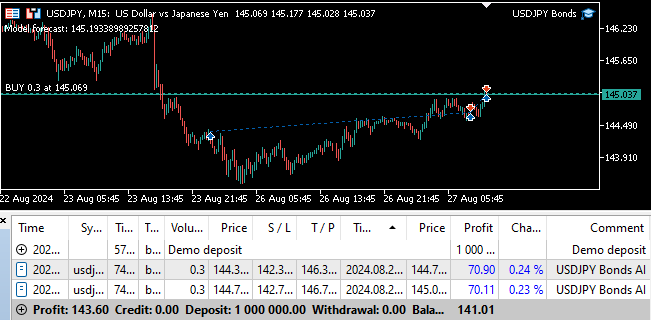
Fig 24: Forward testing our program.

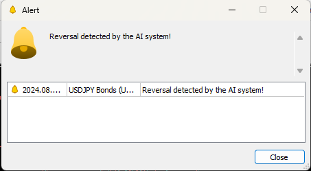
Fig 25: Our Expert Advisor can close positions automatically whenever it detects a reversal.

Conclusion

In this article, we have demonstrated how you can employ AI to give new life to a classic trading strategy. Whether our strategy is worth its complexity is debatable, we could’ve gotten lower accuracy levels using a simpler model. Therefore, we may reasonably conclude that unless more time is invested in transforming the features to better expose the relationship then we may be better off using a simpler strategy of just the ordinary market quotes.