Example of Causality Network Analysis (CNA) and Vector Auto-Regression Model for Market Event Prediction

Introduction

Causality Network Analysis (CNA) is a method used to understand and model complex causal relationships between variables in a system. When applied to financial markets, it can help identify how different market events and factors influence each other, potentially leading to more accurate predictions.

Causal Discovery: Causal discovery is the process of inferring causal relationships from observational data. In the context of financial markets, this means identifying which variables (like economic indicators, market prices, or external events) have causal effects on others. There are several algorithms for causal discovery, but one of the most popular is the PC (Peter-Clark) algorithm.

This trading bot doesn't explicitly implement a system called "Causality Network Analysis for Market Event Prediction" as a named component. However, the bot does incorporate elements of causal analysis and network-based approaches that are conceptually similar. Let's break this down:

Causal Analysis: The bot uses a causal discovery algorithm, specifically the Fast Causal Inference (FCI) algorithm (instead of PC algorithm). This is implemented in the FCIAlgorithm() function.

Network Analysis: The bot uses a network structure to represent relationships between different financial instruments or indicators. This is evident from the Node struct and the SetupNetwork() function.

Event Prediction: While not explicitly called "event prediction", the bot uses a Vector Autoregression (VAR) model to make predictions about future market states. This is implemented in functions like TrainVARModel() and PredictVARValue() .

Causality Network Analysis: A New Frontier in Market Event Prediction

In the world of algorithmic trading, a new approach is gaining traction among quants and traders alike: Causality Network Analysis for Market Event Prediction. This sophisticated method combines the power of causal inference, network theory, and predictive analytics to forecast significant market events with unprecedented accuracy.

Imagine the financial market as a vast, interconnected web. Each strand represents a relationship between different market variables - stock prices, economic indicators, geopolitical events, and more. Traditional analysis often focuses on correlations, but as any seasoned trader knows, correlation doesn't always imply causation.

This is where Causality Network Analysis steps in. It aims to uncover the true cause-and-effect relationships within this complex web. By doing so, it provides traders with a deeper understanding of market dynamics, allowing them to anticipate events that might be invisible to conventional analysis.

At its core, Causality Network Analysis involves three key steps:

1. Building the Network: First, we construct a network where each node represents a market variable. These could be anything from asset prices and trading volumes to economic indicators and sentiment scores.

2. Discovering Causal Links: Next, we use advanced algorithms to determine the causal relationships between these nodes. This is where the magic happens - we're not just looking at which variables move together, but which ones actually drive changes in others.

3. Predicting Events: Finally, we use this causal network to forecast significant market events. By understanding the true drivers of market movements, we can better anticipate major shifts, crashes, or rallies.

The Advantages for Traders

For MQL5 traders, implementing Causality Network Analysis can be a game-changer. Here's why:

• Improved Risk Management: By identifying the root causes of market volatility, you can better prepare for potential downturns.
• More Accurate Predictions: Understanding causal relationships leads to more reliable forecasts than those based on mere correlations.
• Uncovering Hidden Opportunities: The causal network might reveal connections that aren't obvious at first glance, leading to unique trading opportunities.
• Adaptive Strategies: As the market evolves, so does the causal network, allowing your strategies to adapt in real-time.

Implementing in MQL5

While implementing a full Causality Network Analysis system is complex, MQL5 provides a robust platform for this kind of advanced analysis. You might start by:

1. Using the `iCustom()` function to create indicators for each node in your network.
2. Implementing causal discovery algorithms like the PC algorithm or Granger Causality tests (in this case we used FCI algorithms).
3. Leveraging MQL5's neural network capabilities to build predictive models based on your causal network.

Why did we use FCI instead of PC?

FCI (Fast Causal Inference) and PC (Peter-Clark) are both causal discovery algorithms used in the field of causal inference. They're designed to infer causal relationships from observational data. Here's why one might choose FCI over PC:

1. Latent confounders: The main advantage of FCI over PC is its ability to handle latent confounders. FCI can infer the presence of hidden common causes, while PC assumes causal sufficiency (no latent confounders).
2. Selection bias: FCI can also account for selection bias in the data, which PC cannot.
3. More general model: FCI produces a more general graphical model called a Partial Ancestral Graph (PAG), which can represent a broader class of causal structures than the Directed Acyclic Graphs (DAGs) produced by PC.
4. Soundness and completeness: FCI is sound and complete for the class of causally insufficient systems, meaning it can correctly identify all possible causal relationships given infinite sample size.
5. Robustness: Due to its ability to handle latent confounders and selection bias, FCI is generally more robust when dealing with real-world data where hidden variables are common.

However, it's worth noting that FCI has some drawbacks compared to PC:

1. Computational complexity: FCI is generally more computationally expensive than PC, especially for large datasets.
2. Less definitive output: The PAGs produced by FCI often contain more undetermined edge directions than the DAGs from PC, reflecting the additional uncertainty from potential latent confounders.
3. Interpretation: PAGs can be more challenging to interpret than DAGs for non-experts.

In practice, the choice between FCI and PC often depends on the specific requirements of your causal inference task, the nature of your data, and your assumptions about the causal system. If you're confident that there are no hidden confounders and no selection bias, PC might be sufficient and more efficient. If you suspect latent variables or selection bias, FCI would be the more appropriate choice.

Vector Autoregression (VAR) Model

VAR is a multivariate forecasting algorithm that's used when two or more time series influence each other. In this trading system, it's likely used to model the relationships between different financial instruments or economic indicators.

Key features of VAR:

1. It captures linear interdependencies among multiple time series.
2. Each variable is a linear function of past lags of itself and past lags of the other variables.
3. It allows for rich dynamics in a multiple time series system.

In the context of this trading system:

• The VAR model is trained using the `TrainVARModel` function.
• The `PredictVARValue` function uses the trained model to make predictions.
• The system optimizes the VAR model by selecting the optimal lag and significant variables using the `OptimizeVARModel` function.

Mathematical representation:

For a two-variable VAR model with lag 1:

y1,t = c1 + φ11y1,t-1 + φ12y2,t-1 + ε1,t

y2,t = c2 + φ21y1,t-1 + φ22y2,t-1 + ε2,t

Where:

• y1,t and y2,t are the values of the two variables at time t
• c1 and c2 are constants
• φij are the coefficients
• ε1,t and ε2,t are error terms

The system estimates these coefficients to make predictions.

Imagine you're not just predicting the future price of a single asset, but simultaneously forecasting multiple interrelated financial variables. That's where VAR shines. It's like having a crystal ball that doesn't just show you one future, but multiple interconnected futures at once.

At its core, VAR is a multivariate forecasting algorithm used when two or more time series influence each other. In simpler terms, it's a way to capture the linear dependencies among multiple time series.

How Does VAR Work Its Magic?

Let's break it down:

1. Data Collection: You start by gathering historical data for all the variables you want to include in your model. This could be price data for multiple currency pairs, commodities, or even economic indicators.
2. Model Specification: You decide how many lags (past time periods) to include. This is where your trading experience comes in handy!
3. Estimation: The model estimates how each variable is influenced by its own past values and the past values of other variables.
4. Forecasting: Once estimated, the VAR model can generate forecasts for all included variables simultaneously.

Implementing VAR in MQL5

While MQL5 doesn't have a built-in VAR function, you can implement it yourself. Here's a simplified example of how you might structure your code:

// Define your VAR model
struct VARModel {
    int lag;
    int variables;
    double[][] coefficients;
};

// Estimate VAR model
VARModel EstimateVAR(double[][] data, int lag) {
    // Implement estimation logic here
    // You might use matrix operations for efficiency
}

// Make predictions
double[] Forecast(VARModel model, double[][] history) {
    // Implement forecasting logic here
}

// In your EA or indicator
void OnTick() {
    // Collect your multivariate data
    double[][] data = CollectData();
    
    // Estimate model
    VARModel model = EstimateVAR(data, 5); // Using 5 lags
    
    // Make forecast
    double[] forecast = Forecast(model, data);
    
    // Use forecast in your trading logic
    // ...
}

The VAR Advantage in Action

Imagine you're trading EUR/USD. A traditional approach might just look at past EUR/USD prices. But with VAR, you could include:

• EUR/USD prices
• USD/JPY prices (to capture overall USD strength)
• Oil prices (a significant factor for many currencies)
• S&P 500 index (to gauge overall market sentiment)
• US-EU interest rate differential

Now your model captures a much richer picture of the forex landscape, potentially leading to more informed trading decisions.

Challenges and Considerations

Like any powerful tool, VAR comes with its challenges:

1. Data Requirements: VAR models can be data-hungry. Ensure you have sufficient historical data for reliable estimates.
2. Computational Intensity: As you increase variables and lags, computational requirements grow. Optimize your code for efficiency.
3. Stationarity: VAR assumes stationary time series. You might need to pre-process your data (e.g., differencing) to meet this assumption.
4. Interpretation: With multiple variables and lags, interpreting VAR results can be complex. Don't forget to combine statistical insights with your trading knowledge.

Network Analysis in the CNA Trading System

The network analysis implemented in this Expert Advisor (EA) is a fundamental component of its market analysis and prediction strategy. It's designed to represent and analyze the complex relationships between different financial instruments or market variables.

To summarize the key points about the network analysis used in this EA:

1. Structure: The network is composed of nodes, each representing a financial instrument (typically a currency pair).
2. Purpose: It's designed to model the relationships and interdependencies between different financial instruments in the market.
3. Causal Discovery: The EA uses the Fast Causal Inference (FCI) algorithm to uncover potential causal relationships between these instruments.
4. Representation: These relationships are represented in an adjacency matrix, which shows which instruments are directly linked in terms of causal influence.
5. Analysis: The EA performs various analyses on this network, including identifying v-structures (a specific pattern in causal graphs) and applying orientation rules to further refine the understanding of causal relationships.
6. Integration with Prediction: The network structure and the relationships discovered through this analysis serve as inputs for the Vector Autoregression (VAR) model, which is used for making predictions.
7. Adaptive Nature: The network analysis is not static. It can be updated over time, allowing the EA to adapt to changing market conditions and relationships between instruments.

The key idea behind this approach is that financial instruments don't move in isolation. By modeling and analyzing the network of relationships between different instruments, the EA aims to gain a more comprehensive understanding of market dynamics. This, in theory, should lead to more accurate predictions and better-informed trading decisions.

However, it's important to note that while this approach is sophisticated, financial markets are extremely complex and influenced by many factors. The effectiveness of this network analysis would depend on how well it captures real market dynamics and how it's integrated with other components of the trading strategy.

Structure of the Network

The network is represented by the following structures:

struct Node
{
    string name;
    double value;
};

Node g_network[];
int g_node_count = 0;

Each Node in the network represents a specific financial instrument or market variable. The name field identifies the instrument (e.g., "EURUSD", "GBPUSD"), and the value field can store relevant data for that node.

Setting Up the Network

The network is initialized in the SetupNetwork() function:

void SetupNetwork()
{
    string symbols[] = {"EURUSD", "GBPUSD", "USDCAD", "USDCHF", "USDJPY", "AUDUSD"};
    for(int i = 0; i < ArraySize(symbols); i++)
    {
        AddNode(symbols[i]);
    }
}

void AddNode(string name)
{
    ArrayResize(g_network, g_node_count + 1);
    g_network[g_node_count].name = name;
    g_network[g_node_count].value = 0; // Initialize with default value
    g_node_count++;
}

This setup creates a network where each node represents a different currency pair.

Purpose of the Network

The network serves several key purposes in this EA:

1. Representation of Market Structure: It models the interconnections between different currency pairs, allowing the EA to consider how movements in one pair might affect others.
2. Basis for Causal Analysis: The network structure is used as a foundation for the Fast Causal Inference (FCI) algorithm, which attempts to discover causal relationships between the nodes.
3. Input for Predictive Modeling: The network structure and the relationships discovered through causal analysis serve as inputs for the Vector Autoregression (VAR) model used for predictions.

Network Analysis in Action

The EA performs several types of analysis on this network:

1. Causal Discovery: The FCIAlgorithm() function applies the Fast Causal Inference algorithm to uncover potential causal relationships between the nodes.
2. Adjacency Matrix: The causal relationships are represented in an adjacency matrix, where each entry indicates whether there's a direct causal link between two nodes.
3. V-Structure Orientation: The OrientVStructures() function identifies and orients v-structures in the network, which are important patterns in causal graphs.
4. Graph Analysis: The final graph structure is analyzed to inform trading decisions, with the assumption that causally linked instruments may provide predictive information for each other.

Implications for Trading

This network-based approach allows the EA to:

1. Consider complex market dynamics that might not be apparent when looking at instruments in isolation.
2. Potentially identify leading indicators among the analyzed instruments.
3. Make more informed predictions by considering the broader market context.
4. Adapt to changing market conditions as the causal structure is periodically reassessed.

By leveraging this network analysis, the EA aims to gain a deeper understanding of market dynamics, potentially leading to more accurate predictions and better-informed trading decisions.

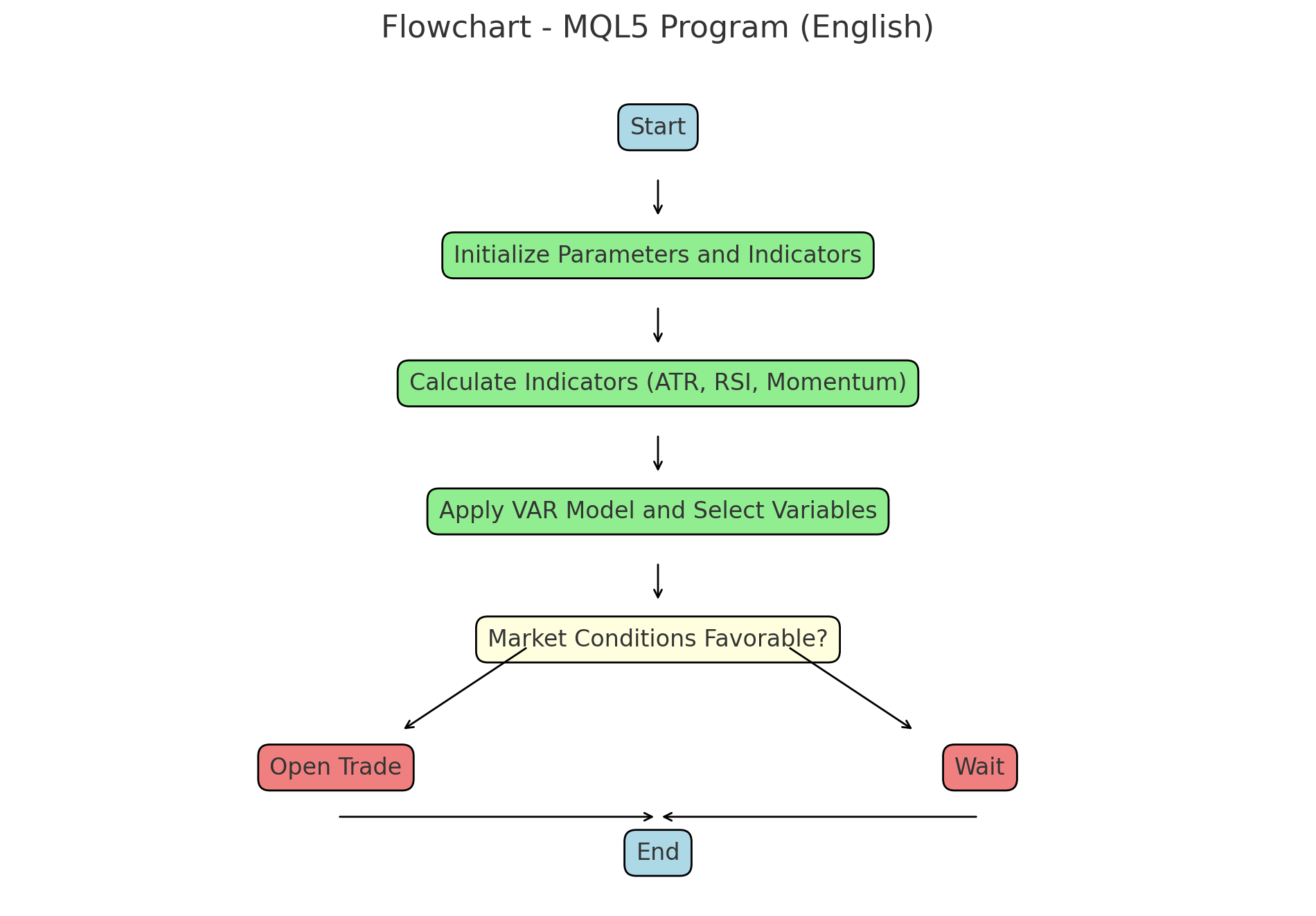
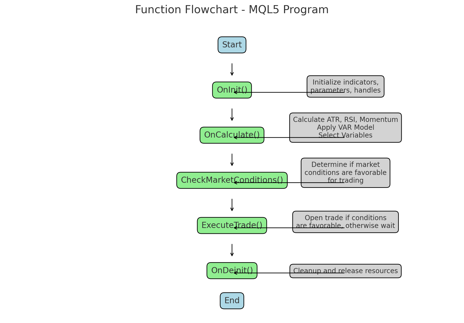
Example Code

This code follows this two flow diagrams:

Detailed Explanation of Key Functions in MQL5 Trading Program

This trading EA is quite sophisticated and combines several advanced approaches:

1. It uses a Vector Autoregression (VAR) model for predictions.
2. It implements a causal discovery algorithm (FCI - Fast Causal Inference) to understand relationships between different market variables.
3. It employs a network structure to represent and analyze multiple financial instruments simultaneously.
4. It incorporates various technical filters such as volatility, RSI, and trend strength.
5. It uses adaptive risk management and position sizing.
6. It implements a sliding window strategy to continuously update and retrain the model.
7. It includes cross-validation and model optimization techniques.

The EA's structure allows for complex analysis and decision-making while maintaining flexibility for future improvements or adaptations to different market conditions.

Detailed Explanation of Key Functions in Trading EA

1. OnInit()

int OnInit()
  {
// Step 1: Set up your network structure
   SetupNetwork();

// Step 2: Run the causal discovery algorithm (e.g., PC or FCI)
   FCIAlgorithm();

// Step 3: Train the optimized causal model
   TrainOptimizedVARModel();

   ArrayResize(g_previous_predictions, g_node_count);
   ArrayInitialize(g_previous_predictions, 0);  // Initialize with zeros

   return(INIT_SUCCEEDED);
  }

This is the initialization function that runs when the EA is first loaded or reloaded on a chart.

Key responsibilities:

• Sets up the network structure by calling SetupNetwork()
• Runs the causal discovery algorithm (FCI) with FCIAlgorithm()
• Trains the optimized causal model using TrainOptimizedVARModel()
• Initializes the array of previous predictions

This function lays the groundwork for all the analysis and prediction the EA will perform.

2. OnTick()

void OnTick()
  {
   ENUM_TIMEFRAMES tf = ConvertTimeframe(InputTimeframe);

   static datetime lastBarTime = 0;
   datetime currentBarTime = iTime(Symbol(), tf, 0);

   if(currentBarTime == lastBarTime)
      return;

   lastBarTime = currentBarTime;

   Print("--- New bar on timeframe ", EnumToString(tf), " ---");

   UpdateModelSlidingWindow();

   for(int i = 0; i < g_node_count; i++)
     {
      string symbol = g_network[i].name;
      Print("Processing symbol: ", symbol);

      double prediction = PredictVARValue(i);
      Print("Prediction for ", symbol, ": ", prediction);

      int signal = GenerateSignal(symbol, prediction);
      Print("Signal for ", symbol, ": ", signal);

      // Imprimir más detalles sobre las condiciones
      Print("RSI: ", CustomRSI(symbol, ConvertTimeframe(InputTimeframe), 14, PRICE_CLOSE, 0));
      Print("Trend: ", DetermineTrend(symbol, ConvertTimeframe(InputTimeframe)));
      Print("Trend Strong: ", IsTrendStrong(symbol, ConvertTimeframe(InputTimeframe)));
      Print("Volatility OK: ", VolatilityFilter(symbol, ConvertTimeframe(InputTimeframe)));
      Print("Fast MA > Slow MA: ", (iMA(symbol, PERIOD_CURRENT, 14, 0, MODE_EMA, PRICE_CLOSE) > iMA(symbol, PERIOD_CURRENT, 24, 0, MODE_EMA, PRICE_CLOSE)));

      if(signal != 0)
        {
         Print("Attempting to execute trade for ", symbol);
         ExecuteTrade(symbol, signal);
        }
      else
        {
         g_debug_no_signal_count++;
         Print("No trade signal generated for ", symbol, ". Total no-signal count: ", g_debug_no_signal_count);
        }
      ManageOpenPositions();
      ManageExistingOrders(symbol);


      Print("Current open positions for ", symbol, ": ", PositionsTotal());
      Print("Current pending orders for ", symbol, ": ", OrdersTotal());
     }

   Print("--- Bar processing complete ---");
   Print("Total no-signal count: ", g_debug_no_signal_count);
   Print("Total failed trade count: ", g_debug_failed_trade_count);
  }

This function is called on each market tick.

Main tasks:

• Converts the input timeframe
• Updates the model using a sliding window with UpdateModelSlidingWindow()
• For each symbol in the network:
  • Predicts values using PredictVARValue()
  • Generates trading signals with GenerateSignal()
  • Executes trades if signals are generated
  • Manages open positions
  • Manages existing orders

This is the operational heart of the EA, where trading decisions are made.

3. OnCalculate()

While not explicitly shown in the provided code, this function would typically be used to calculate custom indicator values. In this EA, some of this functionality seems to be integrated into OnTick().

4. CheckMarketConditions()

int GenerateSignal(string symbol, double prediction)
  {
   int node_index = FindNodeIndex(symbol);
   if(node_index == -1)
      return 0;

   static bool first_prediction = true;
   if(first_prediction)
     {
      first_prediction = false;
      return 0; // No generar señal en la primera predicción
     }

   double current_price = SymbolInfoDouble(symbol, SYMBOL_BID);

// Calculate predicted change as a percentage
   double predicted_change = (prediction - current_price) / current_price * 100;

   bool volatility_ok = VolatilityFilter(symbol, ConvertTimeframe(InputTimeframe));
   double rsi = CustomRSI(symbol, ConvertTimeframe(InputTimeframe), 14, PRICE_CLOSE, 0);
   bool trend_strong = IsTrendStrong(symbol, ConvertTimeframe(InputTimeframe));
   int trend = DetermineTrend(symbol, ConvertTimeframe(InputTimeframe));

   double fastMA = iMA(symbol, PERIOD_CURRENT, 8, 0, MODE_EMA, PRICE_CLOSE);
   double slowMA = iMA(symbol, PERIOD_CURRENT, 24, 0, MODE_EMA, PRICE_CLOSE);

   Print("Debugging GenerateSignal for ", symbol);
   Print("Current price: ", current_price);
   Print("Prediction diff: ", prediction);
   Print("predicted_change: ", predicted_change);
   Print("RSI: ", rsi);
   Print("Trend: ", trend);
   Print("Trend Strong: ", trend_strong);
   Print("Volatility OK: ", volatility_ok);
   Print("Fast MA: ", fastMA, ", Slow MA: ", slowMA);

   bool buy_condition =  prediction >  0.00001 && rsi < 30 && trend_strong  && volatility_ok && fastMA > slowMA;
   bool sell_condition = prediction < -0.00001 && rsi > 70 && trend_strong && volatility_ok && fastMA < slowMA;

   Print("Buy condition met: ", buy_condition);
   Print("Sell condition met: ", sell_condition);

// Buy conditions
   if(buy_condition)
     {
      Print("Buy signal generated for ", symbol);
      int signal = 1;
      return signal;  // Buy signal
     }
// Sell conditions
   else
      if(sell_condition)
        {
         Print("Sell signal generated for ", symbol);
         int signal = -1;
         return signal; // Sell signal
        }
      else
        {
         Print("No signal generated for ", symbol);
         int signal = 0;
         return signal; // No signal
        }


  }

This function is not explicitly defined in the code, but its functionality is distributed across several parts, mainly within GenerateSignal():

• Checks volatility with VolatilityFilter()
• Checks RSI
• Verifies trend strength with IsTrendStrong()
• Determines trend direction with DetermineTrend()
• Compares fast and slow moving averages

These checks determine whether market conditions are favorable for trading.

5. ExecuteTrade()

void ExecuteTrade(string symbol, int signal)
  {
   if(!IsMarketOpen(symbol) || !IsTradingAllowed())
     {
      Print("Market is closed or trading is not allowed for ", symbol);
      return;
     }

   double price = (signal == 1) ? SymbolInfoDouble(symbol, SYMBOL_ASK) : SymbolInfoDouble(symbol, SYMBOL_BID);

   double stopLoss, takeProfit;
   CalculateAdaptiveLevels(symbol, signal, stopLoss, takeProfit);

   double lotSize = CalculateDynamicLotSize(symbol, stopLoss);

   if(lotSize <= 0)
     {
      Print("Invalid lot size for symbol: ", symbol);
      return;
     }

   trade.SetExpertMagicNumber(123456);
   trade.SetTypeFilling(ORDER_FILLING_FOK);

   bool result = false;
   int attempts = 3;

   for(int i = 0; i < attempts; i++)
     {
      if(signal == 1)
        {
         result = trade.Buy(lotSize, symbol, price, stopLoss, takeProfit, "CNA Buy");
         Print("Attempting Buy order: Symbol=", symbol, ", Lot Size=", lotSize, ", Price=", price, ", SL=", stopLoss, ", TP=", takeProfit);
        }
      else
         if(signal == -1)
           {
            result = trade.Sell(lotSize, symbol, price, stopLoss, takeProfit, "CNA Sell");
            Print("Attempting Sell order: Symbol=", symbol, ", Lot Size=", lotSize, ", Price=", price, ", SL=", stopLoss, ", TP=", takeProfit);
           }

      if(result)
        {
         Print("Order executed successfully for ", symbol, ", Type: ", (signal == 1 ? "Buy" : "Sell"), ", Lot size: ", lotSize);
         break;
        }
      else
        {
         int lastError = GetLastError();
         Print("Attempt ", i+1, " failed for ", symbol, ". Error: ", lastError, " - ", GetErrorDescription(lastError));

         if(lastError == TRADE_RETCODE_REQUOTE || lastError == TRADE_RETCODE_PRICE_CHANGED || lastError == TRADE_RETCODE_INVALID_PRICE)
           {
            price = (signal == 1) ? SymbolInfoDouble(symbol, SYMBOL_ASK) : SymbolInfoDouble(symbol, SYMBOL_BID);
            CalculateAdaptiveLevels(symbol, signal, stopLoss, takeProfit);
           }
         else
            break;
        }
     }

   if(!result)
     {
      Print("All attempts failed for ", symbol, ". Last error: ", GetLastError(), " - ", GetErrorDescription(GetLastError()));
     }
  }

This function handles the actual execution of trades.

Key aspects:

• Verifies if the market is open and trading is allowed
• Calculates adaptive stop loss and take profit levels
• Determines lot size based on risk management
• Attempts to execute the order, with retries on failure
• Handles errors and provides detailed feedback

6. OnDeinit()

void OnDeinit(const int reason)
  {
   if(atr_handle != INVALID_HANDLE)
      IndicatorRelease(atr_handle);
   if(rsi_handle != INVALID_HANDLE)
      IndicatorRelease(rsi_handle);
   if(momentum_handle != INVALID_HANDLE)
      IndicatorRelease(momentum_handle);
   GenerateFinalSummary();
  }

This function is called when the EA is removed from the chart or when the terminal is closed.

Main responsibilities:

• Releases indicator handles
• Generates a final summary of the EA's performance by calling GenerateFinalSummary()

Additional Important Functions

UpdateModelSlidingWindow()

void UpdateModelSlidingWindow()
  {
   static int bars_since_update = 0;
   ENUM_TIMEFRAMES tf = ConvertTimeframe(InputTimeframe);

// Check if it's time to update
   if(bars_since_update >= g_update_frequency)
     {
      // Collect new data
      double training_data[];
      CollectTrainingData(training_data, g_window_size, tf);

      // Retrain model
      TrainModel(training_data);

      // Validate model
      double validation_score = ValidateModel();
      Print("Model updated. Validation score: ", validation_score);

      bars_since_update = 0;
     }
   else
     {
      bars_since_update++;
     }
  }

Updates the VAR model using a sliding window of data, allowing the model to adapt to changing market conditions.

TrainOptimizedVARModel()

void TrainOptimizedVARModel()
  {
   OptimizationResult opt_result = OptimizeVARModel();

   Print("Lag óptimo encontrado: ", opt_result.optimal_lag);
   Print("AIC: ", opt_result.aic);
   Print("Variables seleccionadas: ", ArraySize(opt_result.selected_variables));

// Usar opt_result.optimal_lag y opt_result.selected_variables para entrenar el modelo final
   TrainVARModel(opt_result.optimal_lag, opt_result.selected_variables);
  }

Optimizes and trains the VAR model, selecting the optimal number of lags and significant variables.

PredictVARValue()

double PredictVARValue(int node_index)
{
   if(node_index < 0 || node_index >= g_node_count)
   {
      Print("Error: Invalid node index: ", node_index);
      return 0;
   }

   double prediction = 0;
   int lag = g_var_params[node_index].lag;

   Print("Predicting for node: ", g_network[node_index].name, ", Lag: ", lag);

   // Retrieve the previous prediction
   double previous_prediction = g_previous_predictions[node_index];

   // Verify if there are enough coefficients
   int expected_coefficients = g_node_count * lag + 1; // +1 for the intercept
   if(ArraySize(g_var_params[node_index].coefficients) < expected_coefficients)
   {
      Print("Error: Not enough coefficients for node ", node_index, ". Expected: ", expected_coefficients, ", Actual: ", ArraySize(g_var_params[node_index].coefficients));
      return 0;
   }

   prediction = g_var_params[node_index].coefficients[0]; // Intercept
   Print("Intercept: ", prediction);

   double sum_predictions = 0;
   double sum_weights = 0;
   double current_price = iClose(g_network[node_index].name, PERIOD_CURRENT, 0);

   for(int l = 1; l <= lag; l++)
   {
      double time_weight = 1.0 - (double)(l-1) / lag; // Time-based weighting
      sum_weights += time_weight;

      double lag_prediction = 0;
      for(int j = 0; j < g_node_count; j++)
      {
         int coeff_index = (l - 1) * g_node_count + j + 1;
         if(coeff_index >= ArraySize(g_var_params[node_index].coefficients))
         {
            Print("Warning: Coefficient index out of range. Skipping. Index: ", coeff_index, ", Array size: ", ArraySize(g_var_params[node_index].coefficients));
            continue;
         }

         double coeff = g_var_params[node_index].coefficients[coeff_index];
         double raw_value = iClose(g_network[j].name, PERIOD_CURRENT, l);

         if(raw_value == 0 || !MathIsValidNumber(raw_value))
         {
            Print("Warning: Invalid raw value for ", g_network[j].name, " at lag ", l);
            continue;
         }

         // Normalize the value as a percentage change
         double normalized_value = (raw_value - current_price) / current_price;

         double partial_prediction = coeff * normalized_value;
         lag_prediction += partial_prediction;

         Print("Lag ", l, ", Node ", j, ": Coeff = ", coeff, ", Raw Value = ", raw_value,
               ", Normalized Value = ", normalized_value, ", Partial prediction: ", partial_prediction);
      }

      sum_predictions += lag_prediction * time_weight;
      Print("Lag ", l, " prediction: ", lag_prediction, ", Weighted: ", lag_prediction * time_weight);
   }

   Print("Sum of weights: ", sum_weights);

   // Calculate the final prediction
   if(sum_weights > 1e-10)
   {
      prediction = sum_predictions / sum_weights;
   }
   else
   {
      Print("Warning: sum_weights is too small (", sum_weights, "). Using raw sum of predictions.");
      prediction = sum_predictions;
   }

   // Calculate the difference between the current prediction and the previous prediction
   double prediction_change = prediction - previous_prediction;

   Print("Previous prediction: ", previous_prediction);
   Print("Current prediction: ", prediction);
   Print("Prediction change: ", prediction_change);

   // Convert the prediction to a percentage change
   double predicted_change_percent = (prediction - current_price) / current_price * 100;

   Print("Final prediction (as percentage change): ", predicted_change_percent, "%");

   // Update the current prediction for the next iteration
   g_previous_predictions[node_index] = prediction;

   // Return the difference in basis points
   return prediction_change * 10000; // Multiply by 10000 to convert to basis points
}

Makes predictions using the trained VAR model, considering historical values and model coefficients.

ManageOpenPositions() and ManageExistingOrders()

void ManageOpenPositions()
  {
   for(int i = PositionsTotal() - 1; i >= 0; i--)
     {
      ulong ticket = PositionGetTicket(i);
      if(PositionSelectByTicket(ticket))
        {
         string symbol = PositionGetString(POSITION_SYMBOL);
         double openPrice = PositionGetDouble(POSITION_PRICE_OPEN);
         double currentPrice = PositionGetDouble(POSITION_PRICE_CURRENT);
         double stopLoss = PositionGetDouble(POSITION_SL);
         ENUM_POSITION_TYPE positionType = (ENUM_POSITION_TYPE)PositionGetInteger(POSITION_TYPE);

         // Implement trailing stop
         if(positionType == POSITION_TYPE_BUY && currentPrice - openPrice > 2 * CustomATR(symbol, PERIOD_CURRENT, 14, 0))
           {
            double newStopLoss = NormalizeDouble(currentPrice - CustomATR(symbol, PERIOD_CURRENT, 14, 0), SymbolInfoInteger(symbol, SYMBOL_DIGITS));
            if(newStopLoss > stopLoss)
              {
               trade.PositionModify(ticket, newStopLoss, 0);
              }
           }
         else
            if(positionType == POSITION_TYPE_SELL && openPrice - currentPrice > 2 * CustomATR(symbol, PERIOD_CURRENT, 14, 0))
              {
               double newStopLoss = NormalizeDouble(currentPrice + CustomATR(symbol, PERIOD_CURRENT, 14, 0), SymbolInfoInteger(symbol, SYMBOL_DIGITS));
               if(newStopLoss < stopLoss || stopLoss == 0)
                 {
                  trade.PositionModify(ticket, newStopLoss, 0);
                 }
              }
        }
     }
  }

void ManageExistingOrders(string symbol)
  {
   for(int i = PositionsTotal() - 1; i >= 0; i--)
     {
      ulong ticket = PositionGetTicket(i);
      if(PositionSelectByTicket(ticket) && PositionGetString(POSITION_SYMBOL) == symbol)
        {
         double stopLoss = PositionGetDouble(POSITION_SL);
         double takeProfit = PositionGetDouble(POSITION_TP);
         double openPrice = PositionGetDouble(POSITION_PRICE_OPEN);
         double currentPrice = PositionGetDouble(POSITION_PRICE_CURRENT);
         ENUM_POSITION_TYPE positionType = (ENUM_POSITION_TYPE)PositionGetInteger(POSITION_TYPE);

         double atr = CustomATR(symbol, PERIOD_CURRENT, 14, 0);
         double newStopLoss, newTakeProfit;

         if(positionType == POSITION_TYPE_BUY)
           {
            newStopLoss = NormalizeDouble(currentPrice - 2 * atr, SymbolInfoInteger(symbol, SYMBOL_DIGITS));
            newTakeProfit = NormalizeDouble(currentPrice + 3 * atr, SymbolInfoInteger(symbol, SYMBOL_DIGITS));
            if(newStopLoss > stopLoss && currentPrice - openPrice > atr)
              {
               trade.PositionModify(ticket, newStopLoss, newTakeProfit);
              }
           }
         else
            if(positionType == POSITION_TYPE_SELL)
              {
               newStopLoss = NormalizeDouble(currentPrice + 2 * atr, SymbolInfoInteger(symbol, SYMBOL_DIGITS));
               newTakeProfit = NormalizeDouble(currentPrice - 3 * atr, SymbolInfoInteger(symbol, SYMBOL_DIGITS));
               if(newStopLoss < stopLoss && openPrice - currentPrice > atr)
                 {
                  trade.PositionModify(ticket, newStopLoss, newTakeProfit);
                 }
              }

         // Implementar cierre parcial
         double profit = PositionGetDouble(POSITION_PROFIT);
         double volume = PositionGetDouble(POSITION_VOLUME);
         if(profit > 0 && MathAbs(currentPrice - openPrice) > 2 * atr)
           {
            double closeVolume = volume * 0.5;
            if(IsValidVolume(symbol, closeVolume))
              {
               ClosePosition(ticket, closeVolume);
              }
           }
        }
     }
  }

Manage open positions and existing orders, implementing strategies like trailing stops and partial closes.

This EA combines traditional technical analysis with advanced statistical modeling (VAR) and machine learning techniques (causal discovery) to make trading decisions. The modular structure allows for easy modification and improvement of individual components.

Results

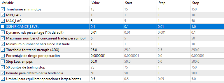
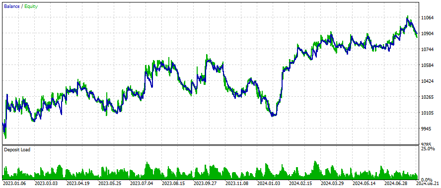
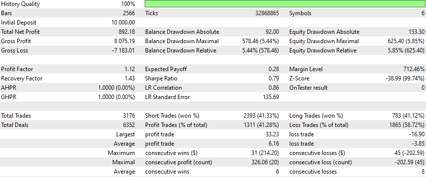
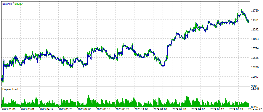
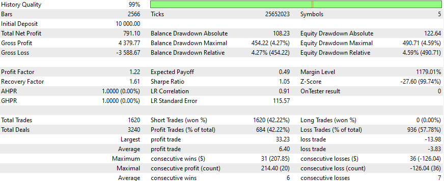
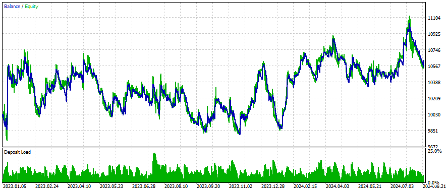
This are the results for some symbols, the settings and inputs will remain the same for all the symbols studied:

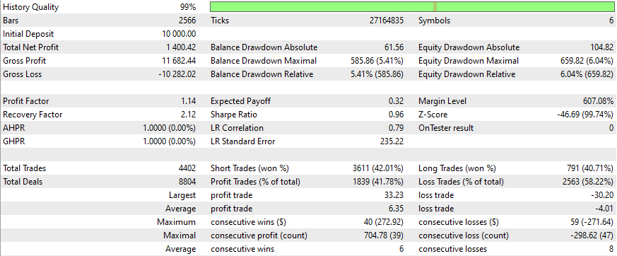
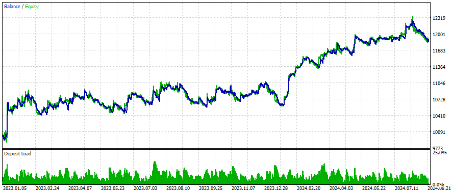
How to get better results?

Better results can be achieved, if in the symbols node you add more and also use co-integrated and correlated symbols. To know which are those symbols, you can use my python script form this article:  Application of Nash's Game Theory with HMM Filtering in Trading - MQL5 Articles.

Also, better results can be achieved if you add to the strategy deep learning. There are some examples of this in articles like this one:  Sentiment Analysis and Deep Learning for Trading with EA and Backtesting with Python - MQL5 Articles 

Also, optimizations have been not done for filters, and you could also try adding more filtering.

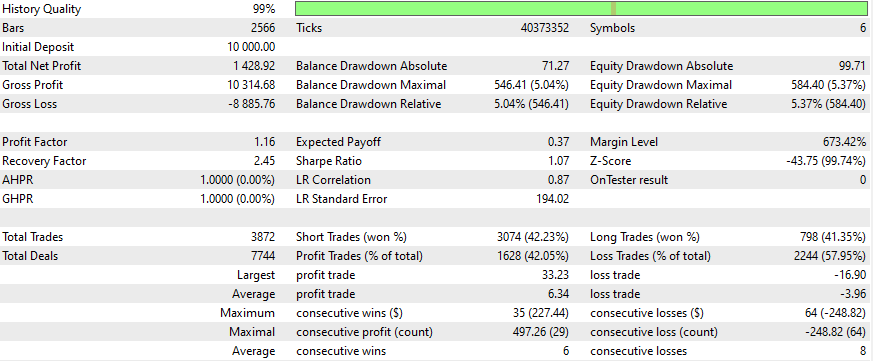
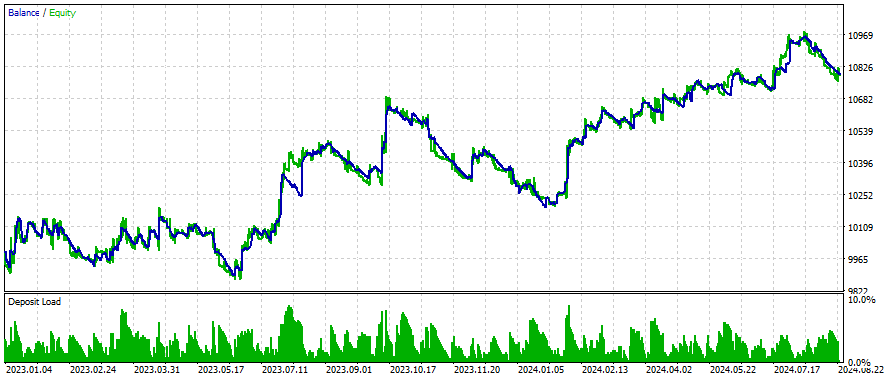
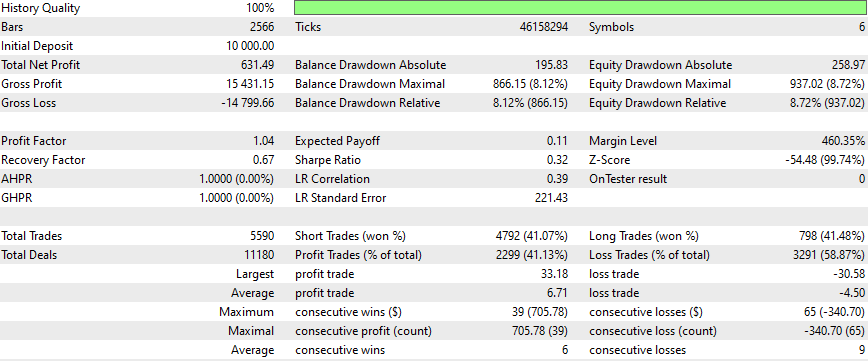
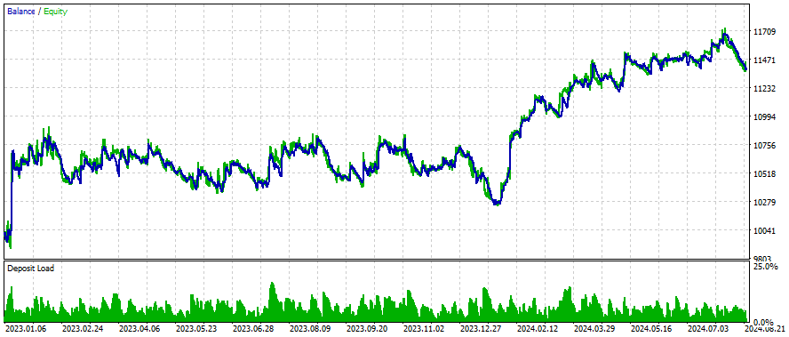
Example of how graph changes with adding more symbols to the network

void SetupNetwork()
  {
   string symbols[] = {"EURUSD", "GBPUSD", "USDCAD", "USDCHF", "USDJPY", "AUDUSD", "XAUUSD", "SP500m", "ND100m"};
   for(int i = 0; i < ArraySize(symbols); i++)
     {
      AddNode(symbols[i]);
     }
  }

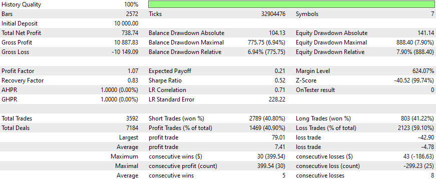
Just adding more symbols to the network, we managed to improve in:

1. Trading activity (more total trades)
2. Short trade win rate
3. Percentage of profitable trades
4. Size of largest profitable trade
5. Average profit per winning trade
6. Lower percentage of losing trades
7. Smaller average loss per losing trade

These improvements suggest better overall trade management and risk control, despite some key performance metrics (like profit factor and recovery factor) being lower.

Conclusion

This article discusses an advanced trading system that integrates Causality Network Analysis (CNA) and Vector Auto-Regression (VAR) for predicting market events and making trading decisions. The system uses sophisticated statistical and machine learning techniques to model relationships between financial instruments. While promising, it emphasizes the importance of combining this approach with robust risk management and a deep understanding of the markets.

For traders seeking better results, the article suggests expanding the network with more correlated symbols, incorporating deep learning, and optimizing filtering methods. Continuous learning and adaptation are crucial for long-term success in trading.

Happy trading, and may your algorithms always stay one step ahead of the market!