Reimagining Classic Strategies (Part IV): SP500 and US Treasury Notes

Introduction

In our previous article, we discussed a potential S&P 500 trading strategy that would rely on us using a selection of stocks that held high weights inside the index. In today's article, we're going to look at an alternative approach of trading the S&P 500 using the Yield of Treasury Notes. For many years now, whenever investors felt risk-adverse, they would normally withdraw their money out of risky investments, such as stocks, and rather save their money in safer investments, such as bonds and treasury notes. Conversely, when investors gained confidence in the markets, they would tend to take their money out of safe investments, such as bonds, and rather invest their money in the stock market.

Fundamental analysts have realized over the years that this correlation between the movements and the S&P 500, and the movement in Treasury Yields seems to be opposing each other. It appears to be a negative correlation, as to say that as investors invested more in stocks, they tend to invest, less in bonds and treasury notes.

Overview of the Trading Strategy

The S&P 500 is a significant benchmark of the performance of America's industrial economy on a very broad level. On the other hand, Treasury notes are considered the safest investments on Earth. When an investor purchases a bond, or a treasury note, they are essentially lending money to the government that issued that treasury note. Each treasury note pays out coupons of interest that are shown on the face of the bond.

When demand for bonds is low, the yield of the bond rises. This is done to rekindle demand. So as fewer investors are buying bonds, we will see the yield rise. In general, fundamental analysts have been using this relationship to their advantage for a long time. If they were trading in the S&P 500, they would look for signs of the trend weakening.

So, for example, if bond yields began to rise, fundamental analysts would know that investors are not buying bonds rather, they may be putting their money into securities that will earn them a higher rate of return, like stocks.

However, if a fundamental analyst noticed that the yield on the bonds has been falling, this is a sign that there's very high demand for bonds. That would tell the fundamental analyst he should probably not invest in the stock market just yet because the general market sentiment is risk-adverse and fundamental strategies would use this to go in and out of their positions.

In today's article, we want to see if this relationship is statistically significant and is it reliable for us to build a trading strategy around this relationship? Let us get started.

Overview of the Methodology

To empirically scrutinize the merits of this strategy, we will fit various models to predict the close price of the SP500 using ordinary OHLC data from the index itself, from there we will observe the change in accuracy when we try to train the models to predict the same target however this time the models will only have access to OHLC data from the USA 5 Year Treasury Note. Our observations led us to believe that investors may be better off using data from the SP500 index. Our model's performance levels dropped across the board, and furthermore, the variance in our error levels increased when we tried using Treasury data. We employed time-series cross validation without random shuffling to compare models of different complexities.

After observing the changes in error levels, we identified the SGD Regressor as the best performing model, we then performed feature selection on the model. None of the data related to the Treasury Notes was selected by our feature selector, indicating the relationship may not be statistically significant. Although at this point we had plenty of evidence that we can drop the Treasury Notes data, we kept the data and continued building our model.

In our final step before exporting the model to ONNX format, we attempted to tune the hyperparameters of the model. We used the L-BFGS-B (Limited-Memory Broyden-Fletcher-Goldfarb-Shanno) algorithm in an attempt to find optimal parameter settings for our model. Our goal was to surpass the performance of the default model settings. Unfortunately, we ended up overfitting our model to the training data and thus failed to outperform the default model.

Exploratory Data Analysis in Python

To fetch data from our MetaTrader 5 Terminal, I created a script to write out historic market data into CSV format for us, I have attached the script along. Simply drag it and drop it on the chart, and it will write out the data for us.

Once the data is prepared, we start off by importing the libraries we need.

#Import the libraries we need 
import pandas as pd
import numpy as np
import seaborn as sns

Once that is done, we will read in our data.

#Read in the data
SP500 = pd.read_csv("/home/volatily/market_data/Market Data US SP 500.csv")
T5Y = pd.read_csv("/home/volatily/market_data/Market Data UST05Y_U4.csv")

We need to define how far into the future we would like to forecast. So in this example, we're going to be forecasting, 20 steps into the future.

#How far into the future should we forecast?
look_ahead = 20

Now, we also have to make sure that the data starts with the oldest day first and the most recent day in the entire data should be lost.

#Make sure the data starts with the oldest day first
SP500 = SP500[::-1].reset_index().set_index("Time").drop(columns=["index"])
T5Y = T5Y[::-1].reset_index().set_index("Time").drop(columns=["index"])

Once that is done, we will now label the data. We will have one label which would be the future close price of the S&P 500, 20 steps into the future. And then the second binary target is only being created for plotting purposes.

#Insert the label
SP500["Target SP500"] = SP500["Close"].shift(-look_ahead)
SP500["Binary Target SP500"] = 0
SP500.loc[SP500["Close"] < SP500["Target SP500"],"Binary Target SP500"] = 1
SP500.dropna(inplace=True)

Now that we have done that, we will merge the two data. We will merge the data on the S&P 500 and the five-year treasury yield into one merge data frame.

#Merge the data
merged_df = pd.merge(SP500,T5Y,how="inner",left_index=True,right_index=True,suffixes=(" SP500"," T5Y"))

And we can observe the merge data frame.

#Let's observe the merged dataframe
merged_df

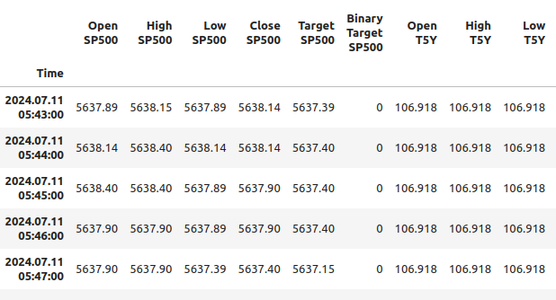
Fig 1: Our merged data frame

We can also analyze the correlation in the merged data frame. We can observe correlation levels are around 0.1, which is not strong.

#Merged data frame correlation
merged_df.corr()

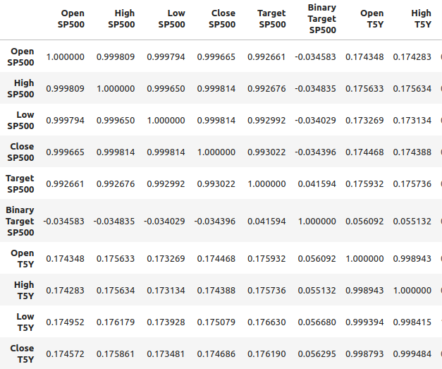
Fig 2: Correlation levels in our merged data frame

However, strong correlation levels do not necessarily imply that there is a definite relationship between the two variables who are looking at. Neither does it imply that one variable is causing the other variable. Strong correlation levels, may imply that there's a common cause that is affecting these two markets.

I did a scatter plot with time on the x-axis, and on the y-axis is the opening price of the S&P 500. And then I used the binary targets to color the points along the scatter plot. Notice that the blue and orange dots naturally cluster together, this may indicate to us that time separates the data well. Recall our binary target tells us what's going to happen 20 steps into the future, blue dots mean the price fell over the next 20 steps and orange dots tell us the opposite happened.

#It appears that one variable that separates the data well is time
sns.scatterplot(data=merged_df,x="Candle",y="Open SP500",hue="Binary Target SP500")

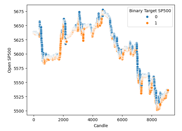
Fig 3: Our data appears to be well separated in time

So it appears that time separates the data very well. However, when we try using other variables to separate the data, like, for example here, we create a scatter plot of the open price of the SP500 against the opening of the five-year treasure yield. We see that we get this poorly separated scatter plot whereby there are so many points on top of each other, and there's no clear separation at all.

#It appears that one variable that separates the data well is time
sns.scatterplot(data=merged_df,x="Open T5Y",y="Open SP500",hue="Binary Target SP500")

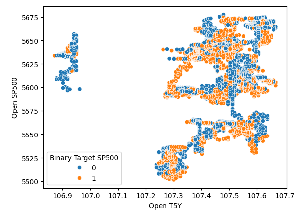
Fig 4: Poor separation levels

Model Selection

Now that we've done that, we will move on to modelling the relationship between the SP500 and Treasury Yields. We will import the modules that we need from scikit-learn.

#Import the libraries we need
from sklearn.linear_model import LinearRegression
from sklearn.linear_model import Lasso
from sklearn.linear_model import SGDRegressor
from sklearn.svm import LinearSVR
from sklearn.ensemble import RandomForestRegressor
from sklearn.ensemble import GradientBoostingRegressor
from sklearn.ensemble import BaggingRegressor
from sklearn.ensemble import AdaBoostRegressor
from sklearn.neural_network import MLPRegressor
from sklearn.model_selection import TimeSeriesSplit
from sklearn.metrics import root_mean_squared_error
from sklearn.preprocessing import RobustScaler
import time
from numpy.random import rand,randn
from scipy.optimize import minimize

And then we will prepare to make a time series split object. So first, we define the number of splits we want, and then we create the time series split object itself.

#Define the number of splits we want
splits = 10

#Create the time series split object
tscv = TimeSeriesSplit(n_splits = splits, gap=look_ahead)

And since we have numerous models, we're going to store them in a list.

#Store the models in a list
models = [LinearRegression(),
         Lasso(),
         SGDRegressor(),
         LinearSVR(),
         RandomForestRegressor(),
         GradientBoostingRegressor(),
         BaggingRegressor(),
         AdaBoostRegressor(),
         MLPRegressor(hidden_layer_sizes=(10,4),early_stopping=True),
         ]

I will define a function to initialize our models, and the function is called "initialize_models".

#Define a function to initialize our models
def initialize_models():
    models = [LinearRegression(),
         Lasso(),
         SGDRegressor(),
         LinearSVR(),
         RandomForestRegressor(),
         GradientBoostingRegressor(),
         BaggingRegressor(),
         AdaBoostRegressor(),
         MLPRegressor(hidden_layer_sizes=(10,4),early_stopping=True),
         ]

And then we also need data frames to store our error levels. So we need three data frames. The first data frame will store our error levels when we are just using ordinary open, high low, close data from the S&P 500, the second data frame stores, our error levels when we are trying to forecast, the S&P 500 just relying on treasury yields. And the last data frame stores our error levels when using all the data we have.

#Create 3 dataframes to measure our performance
#Before we do that, we will define the columns and idexes
columns = ["Linear Regression",
          "Lasso",
          "SGD Regressor",
          "Linear SVR",
          "Random Forest Regressor",
          "Gradient Boosting Regressor",
          "Bagging Regressor",
          "Ada Boost Regressor",
          "MLP Regressor"]
indexes = np.arange(0,10)


#First dataframe stores our error levels using just the ordinary SP500 OHCL
SP500_error = pd.DataFrame(columns=columns,index=indexes)
#Second dataframe stores our error levels using just the ordinary Treasury Yield OHCL
TY5_error = pd.DataFrame(columns=columns,index=indexes)
#Last dataframe stores our error levels using all the data we have
total_error = pd.DataFrame(columns=columns,index=indexes)

We will now define our inputs and our target.

#Now we will define the inputs and target
target = "Target SP500"
predictors = ["Open T5Y",
              "Close T5Y",
              "High T5Y",
              "Low T5Y",
              "Open SP500",
              "Close SP500",
              "High SP500",
              "Low SP500"
             ]

And then we will reset the index of our merged data frame.

#Reset the index
merged_df.reset_index(inplace=True)

And we're going to scale the data using robust scalar. So we simply instantiate the robust scaler, call the transform function and pass the merge data frame to the fit transform function. All of this is wrapped inside a new data frame object that we will create using pandas.

#Scale the data
scaled_data = pd.DataFrame(RobustScaler().fit_transform(merged_df.loc[:,predictors]),columns=predictors,index=np.arange(0,merged_df.shape[0]))

Now that we've come this far, we are now ready to perform cross validation. So the easiest way to have done it was using a nested loop. Therefore, the first for loop is iterating over all the models that we have, and then the second loop will cross validate each model individually. Therefore, we will fit the linear, regression model, then we'll fit the lasso and so on.

#Now we will perform cross validation
#First we iterate over all the models we have
for j in np.arange(0,len(models)):
    for i,(train,test) in enumerate(tscv.split(merged_df)):
        #Prepare the models
        initialize_models()
        #Prepare the data
        X_train = scaled_data.loc[train[0]:train[-1],predictors]
        X_test = scaled_data.loc[test[0]:test[-1],predictors]
        y_train = merged_df.loc[train[0]:train[-1],target]
        y_test = merged_df.loc[test[0]:test[-1],target]
        #Now fit each model and measure its accuracy
        models[j].fit(X_train,y_train)
        SP500_error.iloc[i,j] = root_mean_squared_error(y_test,models[j].predict(X_test))
        print(f"Completed fitting model {models[j]}")

Completed fitting model LinearRegression()
Completed fitting model LinearRegression()
Completed fitting model LinearRegression()
Completed fitting model LinearRegression()
Completed fitting model LinearRegression()

From there, we can see our S&P 500 error levels, and it appears that the linear regression was one of the best performing models in this case, followed by the SGD Regressor. The neural network performed quite poorly. In fact, it could probably benefit a lot from parameter tuning.

SP500_error

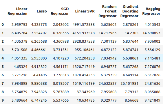
Fig 5: Our error levels when using ordinary OHLC SP500 data

We move on to our five-year treasury yield. In this particular case, all our models performed poorly. However, the Random Forest Regressor appears to perform quite well.

TY5_error

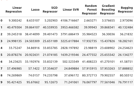
Fig 6: Our error levels when relying on treasury yields

And then, lastly, we have the total error when using all the available data, it appears that the stochastic gradient descent regressor performs reasonably well and so for those reasons, I selected the SGD regressor as the best performing model.

total_error

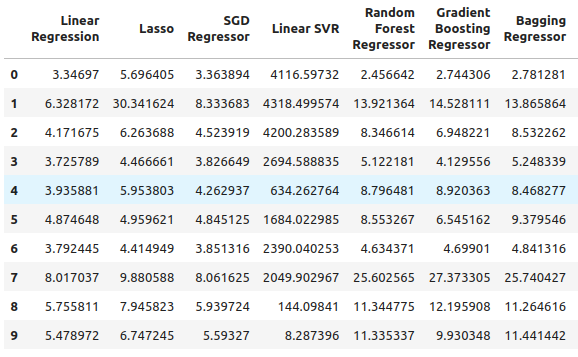
Fig 7: Our error levels when we used all the data available

Feature Selection

We're now going to perform feature selection to see if our computer also thinks that the treasury yield data is important. If the feature selector drops the data related to the treasure yield, then that might be a cause for concern for our strategy because it would appear that the relationship is not reliable. However, if our feature selector retains the treasure yield data, then it might be a good sign.

#Feature selection
from mlxtend.feature_selection import SequentialFeatureSelector as SFS

#Get the best model
model = SGDRegressor()

We create the sequential feature selector object, and we pass it the model that we would like to use. From there, I instructed the algorithm that it can select as many features as necessary. We could have specified that it should select five features, but I wanted to select however many it calculates are important. We set forward to true, so this means it's going to perform forward selection and from there we passed CV equals five, meaning we will employ five-fold cross-validation. From there we passed n-jobs equals minus 1, this allows the feature selector to perform this task in parallel.

#Let us perform feature selection for the best model we have
sfs_sgd_regressor = SFS(model,
                            (1,8),
                            forward=True,
                            cv=5,
                            n_jobs=-1,
                            scoring="neg_mean_squared_error"
                           )

From there, we fit the feature selector.

#Fit the feature selector
sfs_1 = sfs_sgd_regressor.fit(scaled_data.loc[:,predictors],merged_df.loc[:,target])

When we now look at which features were the most important to our model, we see that unfortunately, none of the features related to the treasury. Yields were selected at only selected the close high and low of the S&P 500. So this may indicate that the relationship is not that stable, and it is well known that the correlation between treasury yields and the S&P 500 breaks down from time to time.

#Which features were most important to our model?
sfs_1.k_feature_names_

('Close SP500', 'High SP500', 'Low SP500')

We will still attempt to optimize our model and to see how much performance we can get.

#None the less, let us attempt to optimize the model
from scipy import optimize

And from there, we're going to create going to create two dedicated data sets. One for training and optimizing the model, and the other for validation. On the validation set, we will compare the performance of our optimized model against the performance of a default model that is just using default settings. We want to try to outperform the default error levels.

#Create a training and validation set
scaled_data = merged_df.loc[:,predictors]
scaled_data = (scaled_data - scaled_data.mean()) / (scaled_data.std())
#Create the two datasets
train_data , test_data = scaled_data.loc[:(scaled_data.shape[0]//2),:],scaled_data.loc[(scaled_data.shape[0]//2):,:]

Notice that this time I'm using as a different scaling technique, the first time I just used robust scalar. This time we employed a very common scaling technique whereby we subtract the mean from each column and then divide each column by its standard deviation.

#Let's write out the column mean and standard deviations
#We'll store the mean first 
#Then the standard deviation
scale_factors = pd.DataFrame(columns=predictors,index=(0,1))
#Save the mean and std value of each respective column
for i in (np.arange(0,len(predictors))):
    #Calculate and store the values of each column mean and std
    scale_factors.iloc[0,i] = merged_df.loc[:,predictors[i]].mean()
    scale_factors.iloc[1,i] = merged_df.loc[:,predictors[i]].std()

#Inspect the data
scale_factors

Fig 8: Our mean and standard deviation for each column

The mean values and the standard deviations that we calculated for each column are significant, and we're going to need that data when we're working again in MQL5, so I'm writing out the data into CSV format.

#Write it out to csv format
scale_factors.to_csv("/home/volatily/.wine/drive_c/Program Files/MetaTrader 5/MQL5/Files/sp500_treasury_yields_scale.csv")

Tuning the SGD Regressor Model

We will now attempt to tune the model, we first define the objective function. The objective function in this case will be the training RMSE levels, and we want to minimize our RMSE levels on the training data. However, this procedure is a double-edged sword. Whichever hyperparameters minimize our error on the training set are not guaranteed to minimize our error on the validation set!

#Define the objective function 
def objective(x):
    #Initialize the model with the new parameters
    model = SGDRegressor(alpha=x[0],shuffle=False,eta0=x[1])
    #We need a dataframe to store our current model accuracy levels
    current_accuracy = pd.DataFrame(index=np.arange(0,splits),columns=["Error"])
    #Now we perform cross validation
    for i,(train,test) in enumerate(tscv.split(train_data)):
        #Split the data into a training set and test set
        X_train = train_data.loc[train[0]:train[-1],predictors]
        X_test  = train_data.loc[test[0]:test[-1],predictors]
        y_train = merged_df.loc[train[0]:train[-1],target]
        y_test  = merged_df.loc[test[0]:test[-1],target]
        #Fit the model
        model.fit(X_train,y_train)
        #Record the accuracy
        current_accuracy.iloc[i,0] = root_mean_squared_error(y_test,model.predict(X_test))
    #Return the model accuracrcy
    return(current_accuracy.iloc[:,0].mean())

So, as always, we're going to first start off by performing a line search to an idea of where the optimal values may lie. So we started off by performing just a normal line search, and it took 41 seconds to complete the line search.

#Let's optimize our model
#Let us measure how much time this takes.
start = time.time()

#Create a dataframe to measure the error rates
starting_point_error = pd.DataFrame(index=np.arange(0,21),columns=["Average CV RMSE"])
starting_point_error["Iteration"] = np.arange(0,21)

#Let us first find a good starting point for our optimization algorithm
for i in np.arange(0,21):
    #Set a new starting point
    new_starting_point = (10.0 ** -i)
    #Store error rates
    starting_point_error.iloc[i,0] = objective([new_starting_point  ,new_starting_point]) 

#Record the time stamp at the end
stop = time.time()

#Report the amount of time taken
print(f"Completed in {stop - start} seconds")

Completed in 41.863527059555054 seconds

From the results of our line search, it appears that we crossed over the optimal points right in the first iteration.

starting_point_error["alpha"] = 0
starting_point_error["eta0"] = 0

for i in np.arange(0,21):
    starting_point_error.loc[i,"alpha"] = (10.0 ** -i)
    starting_point_error.loc[i,"eta0"] = (10.0 ** -i)

starting_point_error

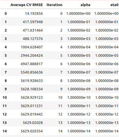
Fig 9: Our line search results

We can also plot this information visually, as you can see it from forms almost an inverted hockey stick with the lowest error at the very beginning and then our error just continues increasing,

#Let's visualize our error levels
sns.lineplot(data=starting_point_error,x="Iteration",y="Average CV RMSE").set(title="Optimizing our SGD Regressor on Training Data")

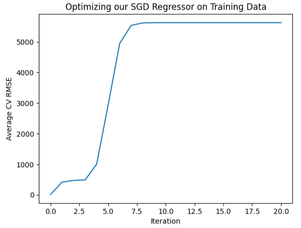
Fig 10: Visualizing our error levels

So now that we have an idea of what appears optimal, we can perform a local search around the region that appears optimal rights. We're going to be using the L-BGFS-B algorithm to find these optimal points. First, we will select random points from the region that appears optimal.

#Now let us perform a local search in the space that appears optimal
pt = abs(((10 ** -2) + rand(2) * ((1) - (10 ** -2))))
pt

array([0.94169659, 0.33068772])

Now we will try to optimize our model to the training data.

#Let's try optimize our model
start = time.time()
bounds = ((0.01,1),(0.01,1))
result = minimize(objective,pt,bounds=bounds,method="L-BFGS-B")
stop = time.time()
print(f"Task completed in {stop - start} seconds")

Task completed in 106.46932244300842 seconds

What are the results?

#What are the results?
result

message: CONVERGENCE: REL_REDUCTION_OF_F_<=_FACTR*EPSMCH
  success: True
   status: 0
      fun: 11.428966326221078
        x: [ 1.040e-01  3.193e-01]
      nit: 24
      jac: [ 9.160e+00 -1.475e+01]
     nfev: 351
     njev: 117
 hess_inv: <2x2 LbfgsInvHessProduct with dtype=float64>

It appears that we were successful, the lowest error we managed to obtain was 11.43, however, the true test comes when we compare the customized model against the default model on the test set.

Testing For Overfitting

To detect if we are overfitting the training data, let us compare the error levels of our customized model with the error levels of a model using default settings. Recall that we partitioned the data set into two halves before we started the parameter tuning process.

#Now let us compare the default model and the customized model
default_model = SGDRegressor()
customized_model = SGDRegressor(alpha=result.x[0],shuffle=False,eta0=result.x[1])

First, let us assess the error levels of the default model and the test set.

#Default model accuracy
default_model.fit(train_data.loc[:,predictors],merged_df.loc[:(merged_df.shape[0]//2),target])
root_mean_squared_error(merged_df.loc[(merged_df.shape[0]//2):,target],default_model.predict(test_data.loc[:,predictors]))

5.793428451043455

Now let us compare that with the error levels of the customized model.

#Customized model accuracy
customized_model.fit(train_data.loc[:,predictors],merged_df.loc[:(merged_df.shape[0]//2),target])
root_mean_squared_error(merged_df.loc[(merged_df.shape[0]//2):,target],customized_model.predict(test_data.loc[:,predictors]))

63.45882351828459

It appears that we were indeed overfitting to the training data, and we failed to outperform the default settings. In this case, we will continue working with the default model and export it to ONNX format.

Exporting to ONNX Format

We start by importing the libraries we need.

#Let's convert the regression model to ONNX format
from skl2onnx.common.data_types import FloatTensorType
from skl2onnx import convert_sklearn
import onnxruntime as ort
import onnx

Then we will normalize and scale our inputs.

for i in predictors:
    merged_df.loc[:,i] = (merged_df.loc[:,i] - merged_df.loc[:,i].mean()) / merged_df.loc[:,i].std()

Now train the model on the entire dataset.

#Prepare the model
model = SGDRegressor()
model.fit(merged_df.loc[:,predictors],merged_df.loc[:,"Target SP500"])

We shall now define the input shape and types.

#Define the input types
initial_type_float = [("float_input",FloatTensorType([1,len(predictors)]))]
onnx_model_float = convert_sklearn(model,initial_types=initial_type_float,target_opset=12)

Let us save the ONNX model.

#ONNX file name
onnx_file_name = "SP500_ONNX_FLOAT_M1.onnx"
#ONNX file
onnx.save_model(onnx_model_float,onnx_file_name)

Now let us quickly inspect the shape of our ONNX model's inputs and outputs.

# load the ONNX model and inspect input and ouput shapes
onnx_session = ort.InferenceSession(onnx_file_name)
input_name = onnx_session.get_inputs()[0].name
output_name = onnx_session.get_outputs()[0].name

Let us ensure that our model input shape is 1 by 8.

#Display information about input tensors in ONNX
print("Information about input tensors in ONNX:")
for i, input_tensor in enumerate(onnx_session.get_inputs()):
    print(f"{i + 1}. Name: {input_tensor.name}, Data Type: {input_tensor.type}, Shape: {input_tensor.shape}")

Information about input tensors in ONNX:
1. Name: float_input, Data Type: tensor(float), Shape: [1, 8]

Lastly, our output shape should be 1 by 1.

#Display information about output tensors in ONNX
print("Information about output tensors in ONNX:")
for i, output_tensor in enumerate(onnx_session.get_outputs()):
    print(f"{i + 1}. Name: {output_tensor.name}, Data Type: {output_tensor.type}, Shape: {output_tensor.shape}")

Information about output tensors in ONNX:
1. Name: variable, Data Type: tensor(float), Shape: [1, 1]

We can also visualize our ONNX model using Netron.

#Visualize the model
import netron

The start function in netron allows us to visualize our ONNX model.

#Call netron 
netron.start(onnx_file_name)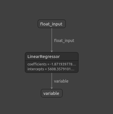

Fig 11: Visualizing our ONNX model using Netron

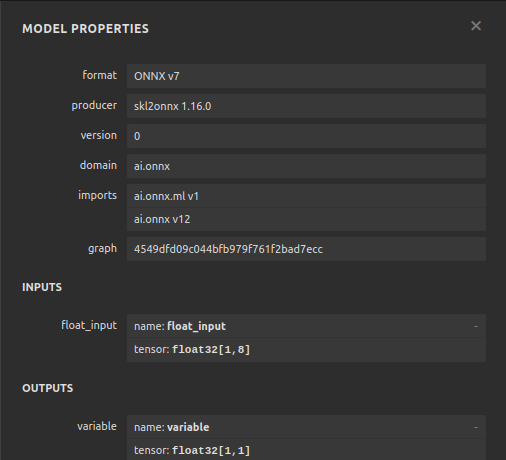
Fig 12: Properties of our ONNX model

Implementation in MQL5

Now that we have finished building our ONNX model, and we've exported it, we can now start building our expert advisor. The first thing we're going to do in our expert advisor is load the ONNX model that we just exported.

//+------------------------------------------------------------------+
//|                                      SP500 X Treasury Yields.mq5 |
//|                                        Gamuchirai Zororo Ndawana |
//|                          https://www.mql5.com/en/gamuchiraindawa |
//+------------------------------------------------------------------+
#property copyright "Gamuchirai Zororo Ndawana"
#property link      "https://www.mql5.com/en/gamuchiraindawa"
#property version   "1.00"
#property tester_file "sp500_treasury_yields_scale.csv"

//+------------------------------------------------------------------+
//| Require the ONNX model                                           |
//+------------------------------------------------------------------+
#resource "\\Files\\SP500_ONNX_FLOAT_M1.onnx" as const uchar ModelBuffer[];

From there we are going to also include the trade library, this library helps us open, close and modify our positions.

//+------------------------------------------------------------------+
//| Libraries we need                                                |
//+------------------------------------------------------------------+
#include <Trade/Trade.mqh>
CTrade Trade;

Also needs to take in some inputs from the end user such as how, big should a lot multiple be and how wide should our stop loss be once that has been done?

//+------------------------------------------------------------------+
//| Inputs for our EA                                                |
//+------------------------------------------------------------------+
input int lot_multiple = 1; //How many times bigger than minimum lot?
input double sl_width = 1;  //How wide should our stop loss be?

We need global variables that will be used throughout the expert advisor. We need one global variable to represent the ONNX model, another vector to store our model's predictions.

//+------------------------------------------------------------------+
//| Global variables                                                 |
//+------------------------------------------------------------------+
long model;                              //Our ONNX SGDRegressor model
vectorf prediction(1);                   //Our model's prediction
float mean_values[8],variance_values[8]; //We need this data to normalise and scale model inputs
double trading_volume;                   //How big should our positions be?
int state = 0;

Moving on, also need of function responsible for reading the CSV config file that we defined earlier. Remember, that file is significant because it contains the mean values and the standard deviation values of each column. This function ensures that all the inputs that we give to our ONNX model are normalized. The function will start off by trying to open the file using the file open command. And if we were successful, and we managed to open the file, we then proceed to parse through our CSV file, and the store the mean values, and the variance values in their own separates arrays. Otherwise, if we're unsuccessful, then the function is going to print that it failed to read the file, and it will return false, and the initialization procedure will fail.

//+------------------------------------------------------------------+
//| A function responsible for reading the CSV config file           |
//+------------------------------------------------------------------+
bool read_configuration_file(void)
  {
//--- Read the config file
   Print("Reading in the config file");

//--- Config file name
   string file_name = "sp500_treasury_yields_scale.csv";

//--- Try open the file
   int result = FileOpen(file_name,FILE_READ|FILE_CSV|FILE_ANSI,",");

//--- Check the result
   if(result != INVALID_HANDLE)
     {
      Print("Opened the file");
      //--- Prepare to read the file
      int counter = 0;
      string value = "";
      //--- Make sure we can proceed
      while(!FileIsEnding(result) && !IsStopped())
        {
         if(counter > 60)
            break;
         //--- Read in the file
         value = FileReadString(result);
         Print("Reading: ",value);
         //--- Have we reached the end of the line?
         if(FileIsLineEnding(result))
            Print("row++");
         counter++;
         //--- The first few lines will contain the title of each columns, we will ingore that
         if((counter >= 11) && (counter <= 18))
           {
            mean_values[counter - 11] = (float) value;
           }
         if((counter >= 20) && (counter <= 27))
           {
            variance_values[counter - 20] = (float) value;
           }
        }
      //--- Close the file
      FileClose(result);
      Print("Mean values");
      ArrayPrint(mean_values);
      Print("Variance values");
      ArrayPrint(variance_values);
      return(true);
     }

   else
      if(result == INVALID_HANDLE)
        {
         Print("Failed to read the file");
         return(false);
        }

   return(false);
  }

We also need a function responsible for getting a forecast from our model. We have a vector at the beginning to store the input data. Once we have fetched all the prices we need, we subtract the mean value for that column and divide by the variance for that particular column. Once that has been done, we can then get a prediction from our model.

//+------------------------------------------------------------------+
//| A function responsible for getting a forecast from our model     |
//+------------------------------------------------------------------+
void predict(void)
  {
//--- Let's prepare our inputs
   vectorf input_data = vectorf::Zeros(8);
//--- Select the symbol
   input_data[0] = ((iOpen("UST05Y_U4",PERIOD_M1,0) - mean_values[0]) / variance_values[0]);
   input_data[1] = ((iClose("UST05Y_U4",PERIOD_M1,0) - mean_values[1]) / variance_values[1]);
   input_data[2] = ((iHigh("UST05Y_U4",PERIOD_M1,0) - mean_values[2]) / variance_values[2]);
   input_data[3] = ((iLow("UST05Y_U4",PERIOD_M1,0) - mean_values[3]) / variance_values[3]);;
   input_data[4] = ((iOpen("US500",PERIOD_M1,0) - mean_values[4]) / variance_values[4]);;
   input_data[5] = ((iClose("US500",PERIOD_M1,0) - mean_values[5]) / variance_values[5]);;
   input_data[6] = ((iHigh("US500",PERIOD_M1,0) - mean_values[6]) / variance_values[6]);
   input_data[7] = ((iLow("US500",PERIOD_M1,0) - mean_values[7]) / variance_values[7]);;
//--- Show the inputs
   Print("Inputs: ",input_data);
//--- Obtain a prediction from our model
   OnnxRun(model,ONNX_DEFAULT,input_data,prediction);
  }

After our model has given us a prediction, we need to take action. So, in this particular case, we can either decide to open a position in the direction that our model has predicted. Or if our model is forecasting that price is going to reverse against us, we might decide to close our open positions.

//+------------------------------------------------------------------+
//| This function will decide if we should open or close our trades  |
//+------------------------------------------------------------------+
void intepret_prediction(void)
  {
   if(PositionsTotal() == 0)
     {
      double ask = SymbolInfoDouble("US500",SYMBOL_ASK);
      double bid = SymbolInfoDouble("US500",SYMBOL_BID);
      double close = iClose("US500",PERIOD_M1,0);
      if(prediction[0] > close)
        {
         Trade.Buy(trading_volume,"US500",ask,(ask - sl_width),(ask + sl_width),"SP500 X Treasury Yields");
         state = 1;
        }

      if(prediction[0] < iClose("US500",PERIOD_M1,0))
        {
         Trade.Sell(trading_volume,"US500",bid,(bid + sl_width),(bid - sl_width),"SP500 X Treasury Yields");
         state = 2;
        }
     }
   else
      if(PositionsTotal() > 0)
        {
         if((state == 1) && (prediction[0] > iClose("US500",PERIOD_M1,0)))
           {
            Alert("Reversal predicted, consider closing your buy position");
           }

         if((state == 2) && (prediction[0] < iClose("US500",PERIOD_M1,0)))
           {
            Alert("Reversal predicted, consider closing your buy position");
           }
        }

  }

We have finished defining the helper functions for our model, and we move on to defining the initialization function of our Expert Advisor. First have to create our ONNX model and then ensure that the model is valid.

//+------------------------------------------------------------------+
//| Expert initialization function                                   |
//+------------------------------------------------------------------+
int OnInit()
  {

//--- Create the ONNX model from the model buffer we have
   model = OnnxCreateFromBuffer(ModelBuffer,ONNX_DEFAULT);

//--- Ensure the model is valid
   if(model == INVALID_HANDLE)
     {
      Comment("[ERROR] Failed to initialize the model: ",GetLastError());
      return(INIT_FAILED);
     }

Once we are confident the model is valid, we define the input shapes of our model, and then we define the output shapes of our model.

//--- Define the model parameters, input and output shapes
   ulong input_shape[] = {1,8};

//--- Check if we were defined the right input shape
   if(!OnnxSetInputShape(model,0,input_shape))
     {
      Comment("[ERROR] Incorrect input shape specified: ",GetLastError(),"\nThe model's inputs are: ",OnnxGetInputCount(model));
      return(INIT_FAILED);
     }

   ulong output_shape[] = {1,1};

//--- Check if we were defined the right output shape
   if(!OnnxSetOutputShape(model,0,output_shape))
     {
      Comment("[ERROR] Incorrect output shape specified: ",GetLastError(),"\nThe model's outputs are: ",OnnxGetOutputCount(model));
      return(INIT_FAILED);
     }

Once all of that is done, we can then read in the configuration file, this has to be done on initialization and if we fail to read the configuration file, the entire expert advisor should terminate because we cannot make forecasts on data that is not normalized.

//--- Read the configuration file
   if(!read_configuration_file())
     {
      Comment("Failed to find the configuration file, ensure it is stored here: ",TerminalInfoString(TERMINAL_DATA_PATH));
      return(INIT_FAILED);
     }

Now we need to select the symbols and add them to the Market Watch.

//--- Select the symbols
   SymbolSelect("US500",true);
   SymbolSelect("UST05Y_U4",true);

Lastly, we need to fetch some market data.

//--- Calculate the lotsize
   trading_volume = SymbolInfoDouble(Symbol(),SYMBOL_VOLUME_MIN) * lot_multiple;

//--- Return init succeeded
   return(INIT_SUCCEEDED);
  }

Whenever our Expert Advisor is not in use, we must free up the resources that were allocated to us.

//+------------------------------------------------------------------+
//| Expert deinitialization function                                 |
//+------------------------------------------------------------------+
void OnDeinit(const int reason)
  {
//--- Free up the resources we used for our ONNX model
   OnnxRelease(model);
//--- Remove the expert advisor
   ExpertRemove();
  }

Finally, in our OnTick event handler, we will make predictions using our ONNX model and then map those predictions into actions.

//+------------------------------------------------------------------+
//| Expert tick function                                             |
//+------------------------------------------------------------------+
void OnTick()
  {
//--- Get a prediction
   predict();
//--- Interpret the forecast
   intepret_prediction();
   Comment("Model forecast",prediction[0]);
  }

Fig 13: Our expert advisor in action

Conclusion

In this article, we revisited the classic SP500 trading strategy that relies on the yield of Treasury Notes. Our analysis has shown that the relationship is not always stable and furthermore, it appears that investors may be better off using ordinary market data from the SP500 index itself.