
The price movement model and its main provisions. (Part 3): Calculating optimal parameters of stock exchange speculations

Introduction
In the previous articles (Part 1 and Part 2), I presented the fundamental principles and latent mechanisms for generating price dynamics, which was purely theoretical in nature and even went beyond the scope of what was observed (being, however, the basis of it). In this and subsequent articles, I will try to lay the foundations of a new engineering discipline (where many calculations will be of an evaluative nature), which would allow users to draw practically useful conclusions from the observed price dynamics and directly apply them in trading. In this article, I will talk about engineering approaches and algorithms that, in general, are able to provide sustainable profits, as well as probabilistic calculations of those optimal take profit and stop loss values that would allow achieving the maximum average profit.1. Model.
In the previous article (Part 2), I obtained the (II.3) equation for the price probability flow (for brevity, from now on, the (N) equation of the Part R article is numbered as (R.N), where R is a Roman numerical). Such a probability flow in reduced or observed form is expressed in "up" and "down" price movement probabilities, or, to be more precise, it creates such probabilities. Let's formulate the approach to the practical assessment of such probabilities.
In the discrete time representation (based on the bar concept), when the ![]() price history segment (Open, Close, High or Low) is presented as the
price history segment (Open, Close, High or Low) is presented as the ![]() series (the numeration order here is so that subsequent bars have higher numbers than that of the previous ones), the price moves in discrete steps. On large scales or in case of the quite large
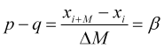
series (the numeration order here is so that subsequent bars have higher numbers than that of the previous ones), the price moves in discrete steps. On large scales or in case of the quite large ![]() , this allows us to discuss the probabilities of such price leaps assessed for the upward price movement probability, as
, this allows us to discuss the probabilities of such price leaps assessed for the upward price movement probability, as ![]() , where
, where ![]() - number of
- number of ![]() set members, or for the downward one
set members, or for the downward one ![]() , where
, where ![]() - number of
- number of ![]() members. At the same time, it is possible to calculate the longevity of the average leap
members. At the same time, it is possible to calculate the longevity of the average leap
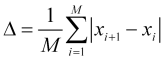 (1.1)
(1.1)
of the ![]() price. In practice, we can find out that a chaotically moving price for the
price. In practice, we can find out that a chaotically moving price for the ![]() period deviates from its current average (defined by such probabilities) due to a random walk. The deviation is of the order of
period deviates from its current average (defined by such probabilities) due to a random walk. The deviation is of the order of
![]() , (1.2)
, (1.2)
(this is confirmed by the Casual Channel indicator whose channel lines are ![]() or deviations (1.2) from the moving average of the
or deviations (1.2) from the moving average of the ![]() period).
period).
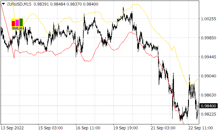
Fig. 1. Casual Channel indicator
Obviously, the characteristic time of the random price deviation by ![]() of the order of
of the order of ![]() , where
, where ![]() is a temporary bar length of the appropriate timeframe. We would see the same deviation (1.2) from the price from the average, if the price randomly moved by similar leaps exactly equal to
is a temporary bar length of the appropriate timeframe. We would see the same deviation (1.2) from the price from the average, if the price randomly moved by similar leaps exactly equal to ![]() .
.
Therefore, in the model simplification provided here, we will assume that the price moves in similar ![]() leaps, with the probabilities of their directions of
leaps, with the probabilities of their directions of ![]() and
and ![]() .
.
The ![]() leap, calculated using the methods described above, as well as the proabilities were already relevant for the previous
leap, calculated using the methods described above, as well as the proabilities were already relevant for the previous ![]() interval as a whole, i.e. as averages for the value range, rather than for the current price movements formed under the influence of different
interval as a whole, i.e. as averages for the value range, rather than for the current price movements formed under the influence of different ![]() leaps and, most importantly,
leaps and, most importantly, ![]() and
and ![]() probabilities that is yet to be forecast.
probabilities that is yet to be forecast.
As I mentioned in Part 2, the methods of conventional statistics and its mathematical apparatus are not suitable in case of the price dynamics formed out of superpositions of the probability waves causing considerable errors. Thus, the analysis based on applying observed data and the appropriate probabilistic and statistic calculations have approximate nature.
2. Practical determination of previously operating probabilities and normalized price velocity. The principle of using these parameters to calculate the future price distribution.
Average speed of price movement over the averaging interval ![]() is equal to
is equal to
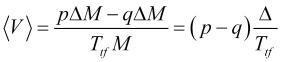 (2.1)
(2.1)
and shows the ![]() moving average change rate (where
moving average change rate (where ![]() is a bar index) with the appropriate averaging period, and not some kind of speed fluctuations. Therefore, the average speed is a practically calculable quantity
is a bar index) with the appropriate averaging period, and not some kind of speed fluctuations. Therefore, the average speed is a practically calculable quantity
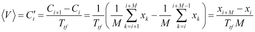 . (2.2)
Equating (2.1) to (2.2), we obtain an empirically determined parameter
 , (2.3)
Let's call this a normalized price speed, since ![]() , while
, while ![]() .
. ![]() is easy to demonstrate. In fact, for example, from (1.1) follows the inequality
is easy to demonstrate. In fact, for example, from (1.1) follows the inequality
 , (2.4)
entailing ![]() together with (2.3). We can also assume
together with (2.3). We can also assume ![]() , and since the probability is
, and since the probability is ![]() , then
, then ![]() . Use (2.3) and
. Use (2.3) and ![]() to find the probabilities
to find the probabilities
![]() and
and ![]() , (2.5)
, (2.5)
as well as another expression for the normalized speed
 , (2.6)
where the parameter
![]() . (2.7)
. (2.7)
In further calculations, we will also need the parameter
 , (2.8)
through which the normalized speed itself is expressed as follows
 . (2.9)
The (2.5) probabilities of leaps calculated on the ![]() price interval are the average ones for the interval and participate in forming the
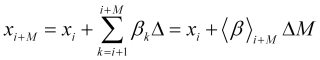
price interval are the average ones for the interval and participate in forming the ![]() end price. Therefore, if we know (at the current moment of
end price. Therefore, if we know (at the current moment of ![]() beforehand when the
beforehand when the ![]() price is known) these average probabilities, we can predict the price
price is known) these average probabilities, we can predict the price ![]() in the future
in the future ![]() , or, to be more precise, the probability distribution
, or, to be more precise, the probability distribution ![]() of the price. When comparing the
of the price. When comparing the ![]() price charts and the
price charts and the ![]() normalized speed (from which
normalized speed (from which ![]() and
and ![]() are calculated), we can trace their strong similarity (by the coincidence of their vertices locations), showing that it was this speed (more precisely, the probabilities corresponding to it) that formed the current price of
are calculated), we can trace their strong similarity (by the coincidence of their vertices locations), showing that it was this speed (more precisely, the probabilities corresponding to it) that formed the current price of ![]() .
.
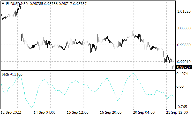
Fig. 2. The figure shows the normalized speed graph.
Indeed, from (2.3) it follows ![]() . This means that the
. This means that the ![]() price is formed from the
price is formed from the ![]() price by the array of future velocities
price by the array of future velocities ![]() or their averages by the interval
or their averages by the interval
 , (2.10)
where the average normalized speed over the future interval, displayed on its graph at the point ![]()
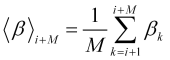 , (2.11)
while the averages of the probability interval ![]() and
and ![]() are found substituting
are found substituting ![]() to the equations (2.5) (obviously, if in (2.10) the
to the equations (2.5) (obviously, if in (2.10) the ![]() member is around
member is around ![]() , then we have the graphs resembling
, then we have the graphs resembling ![]() and
and ![]() ). Then, having predicted sufficiently smooth functions
). Then, having predicted sufficiently smooth functions ![]() on
on ![]() bars forward, we calculate the necessary probabilities
bars forward, we calculate the necessary probabilities ![]() and
and ![]() , which allows us to calculate (at the moment of
, which allows us to calculate (at the moment of ![]() ) the
) the ![]() probability distribution of the
probability distribution of the ![]() future price and its parameters necessary for trading (position opening direction and stop order position).
future price and its parameters necessary for trading (position opening direction and stop order position).
The essence of the normalized speed forecast used here is as follows. The ![]() temporary function of the normalized speed fluctuates within the range of
temporary function of the normalized speed fluctuates within the range of ![]() near its mathematical expectation equal to zero (or the
near its mathematical expectation equal to zero (or the ![]() small value displaying the velocity of the global trend, if it covers the entire area under consideration). In this case, for example, the simplest statistical forecast based on the conditional mathematical expectation taking the form of
small value displaying the velocity of the global trend, if it covers the entire area under consideration). In this case, for example, the simplest statistical forecast based on the conditional mathematical expectation taking the form of ![]() will bring the predictive function closer to zero or
will bring the predictive function closer to zero or ![]() according to
according to ![]() . In other words, as the autocorrelation function of the corresponding process
. In other words, as the autocorrelation function of the corresponding process ![]() decreases sharply reducing the number of positions opened by a condition like
decreases sharply reducing the number of positions opened by a condition like ![]() and making the game even less profitable, than a game with a trivial forecast based on the last value
and making the game even less profitable, than a game with a trivial forecast based on the last value ![]() . On the other hand, price dynamics are well modeled and predicted by oscillatory processes. The idea behind this was revealed in previous articles. At this stage of theory development, the
. On the other hand, price dynamics are well modeled and predicted by oscillatory processes. The idea behind this was revealed in previous articles. At this stage of theory development, the ![]() forecast of the
forecast of the ![]() function (having an oscillatory nature) on
function (having an oscillatory nature) on ![]() bars forward was made based on Fourier extrapolation calculated on the basis of empirical historical data
bars forward was made based on Fourier extrapolation calculated on the basis of empirical historical data ![]() , since the use of the wavelet extrapolation proposed in previous articles in this case has not yet provided noticeable advantages.
, since the use of the wavelet extrapolation proposed in previous articles in this case has not yet provided noticeable advantages.
3. Trend quality. Assessing the extent of current and future trends, adequate work horizon.
If the trend lasts longer than the ![]() averaging time, then the natural increase in price during the averaging time (according to (2.1) and (2.3)) is of the order of
averaging time, then the natural increase in price during the averaging time (according to (2.1) and (2.3)) is of the order of
![]() . (3.1)
. (3.1)
Increment uncertainty
![]() , (3.2)
, (3.2)
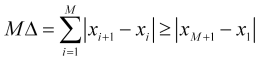
then the full range of price movement (see Fig. 1), when it moves from one border of the Casual Channel indicator channel to another and at the same time drifts on average at the ![]() normalized speed, is estimated as
normalized speed, is estimated as
![]() , (3.3)
, (3.3)
where
![]() . (3.4)
. (3.4)
If we follow the trend, then it is desirable that the value of the shift (3.1) remains significantly greater than the uncertainty (3.2) of this shift
![]() , (3.5)
, (3.5)
from it and from (2.6) and (2.9), we obtain a lower estimate for the required averaging time
 , (3.6)
when fulfilled, in accordance with (3.4), the averaging time (in bars) is calculated as
 . (3.7)
If the ![]() uncertainty price increment cannot be neglected, then the averaging time is considered as the positive root of the quadratic equation (3.4)
uncertainty price increment cannot be neglected, then the averaging time is considered as the positive root of the quadratic equation (3.4)
 . (3.7.1)
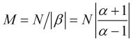
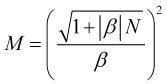
Define the trend quality
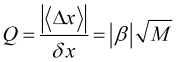 , (3.8)
as the ratio of its natural increment to its uncertainty or noise. It is quite clear that a stable profitable trend-following strategy requires the high ![]() quality. But the Quality Trend indicator calculating the quality (Fig. 3), reaches the value of several units for a currency at best. Moreover, even having identified a high-quality trend, it is not possible to determine when it will end due to the unpredictability of the emergence of strong external events that can disrupt the market’s own dynamics and end the trend or even reverse it. Therefore, a profitable strategy can only be based on taking profits on relatively small fluctuations in the direction of the trend .
quality. But the Quality Trend indicator calculating the quality (Fig. 3), reaches the value of several units for a currency at best. Moreover, even having identified a high-quality trend, it is not possible to determine when it will end due to the unpredictability of the emergence of strong external events that can disrupt the market’s own dynamics and end the trend or even reverse it. Therefore, a profitable strategy can only be based on taking profits on relatively small fluctuations in the direction of the trend .
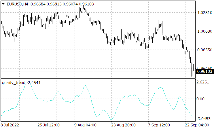
Fig. 3. The Quality Trend indicator where the price increment is not taken modulo, i.e. the sign of the indicator indicates the direction of the trend.
Note that Quality Trend indicator readings being proportional to the normalized speed, as was shown by the (2.10) ratio for it, turn out to be similar to the price history in the positions of their peaks and, accordingly, the Quality Trend readings turn out to not lag behind. Moreover, the indicator readings may surpass (which they often do) price movements, since even before the trend changes, the corresponding speed of a price movement (growth for an uptrend or fall for a downtrend) decreases. However, such predictive behavior of this indicator occurs only in the absence of strong influences on the market that disrupt its own movement. After such influences, during their relaxation time, the Quality Trend readings become "ordinary" lagging ones, with the lag determined by its averaging period.
Let's analyze the behavior of the ![]() function and evaluate the possible extent of trends, provided there are no strong third-party influences on the market. With the decreasing
function and evaluate the possible extent of trends, provided there are no strong third-party influences on the market. With the decreasing ![]() average period, the calculated values
average period, the calculated values ![]() of the normalized velocity may increase (after all, its “instant” values in a constantly changing market change with a greater amplitude than average ones and the greater the averaging, the smaller such variations), i.e. in the quality factor ratio, the members, for which
of the normalized velocity may increase (after all, its “instant” values in a constantly changing market change with a greater amplitude than average ones and the greater the averaging, the smaller such variations), i.e. in the quality factor ratio, the members, for which ![]() and vice versa
and vice versa ![]() are multiplied, which makes it possible for the
are multiplied, which makes it possible for the ![]() function to have maximums. However, on a very small interval, when the true probabilities of
function to have maximums. However, on a very small interval, when the true probabilities of ![]() and
and ![]() leaps are constant, due to small changes in the market situation on it, their statistically calculated values
leaps are constant, due to small changes in the market situation on it, their statistically calculated values ![]() and
and ![]() over this short averaging period, will most likely differ greatly from the true probabilities, because with the uncertainty period decrease, the
over this short averaging period, will most likely differ greatly from the true probabilities, because with the uncertainty period decrease, the ![]() and
and ![]() of the probabilities calculated on it increase. Therefore, for the
of the probabilities calculated on it increase. Therefore, for the ![]() averaging period providing the calculation of more or less reliable probabilities, the
averaging period providing the calculation of more or less reliable probabilities, the ![]() type ratios should be satisfied, which will determine its minimum value. Otherwise, when
type ratios should be satisfied, which will determine its minimum value. Otherwise, when ![]() (although this is a broader case than the case of large fluctuations in the instantaneous normalized velocity at small averaging intervals, since such a ratio can also occur at large intervals with a rapid change in the true probability
(although this is a broader case than the case of large fluctuations in the instantaneous normalized velocity at small averaging intervals, since such a ratio can also occur at large intervals with a rapid change in the true probability ![]() ), statistically calculated probability values cannot be used. Note that in cases of strong fluctuations of the normalized velocity, the
), statistically calculated probability values cannot be used. Note that in cases of strong fluctuations of the normalized velocity, the ![]() function based on it also fluctuates strongly near its maximum, so the maximum used to analyze the market situation should be chosen such that it forms smoothly, which, as follows from the above, is achieved with sufficiently large averaging periods. If the
function based on it also fluctuates strongly near its maximum, so the maximum used to analyze the market situation should be chosen such that it forms smoothly, which, as follows from the above, is achieved with sufficiently large averaging periods. If the ![]() condition is met, which is assumed to be fulfilled in the further theory, the estimated probabilities
condition is met, which is assumed to be fulfilled in the further theory, the estimated probabilities ![]() and
and ![]() can be identified with acting
can be identified with acting ![]() and
and ![]() probabilities, which then we will also write as
probabilities, which then we will also write as ![]() and
and ![]() .
.
Precisely in those areas where the ![]() and
and ![]() probabilities are constant, a stable trend is formed, while the drop in the prevailing probability
probabilities are constant, a stable trend is formed, while the drop in the prevailing probability ![]() (i.e.
(i.e. ![]() ) will reduce the growth rate of the increment
) will reduce the growth rate of the increment ![]() and maybe even (when the inverse relationship
and maybe even (when the inverse relationship ![]() is achieved) reverse the trend, which also leads to a drop in the calculated quality factor. On the contrary, high quality factor and its growth indicate not only a strong predominance of the prevailing probability
is achieved) reverse the trend, which also leads to a drop in the calculated quality factor. On the contrary, high quality factor and its growth indicate not only a strong predominance of the prevailing probability ![]() over
over ![]() , but also about its constancy and even increase. . Therefore, the higher the trend quality (3.8), the greater the probability that it is present there, i.e. over the entire
, but also about its constancy and even increase. . Therefore, the higher the trend quality (3.8), the greater the probability that it is present there, i.e. over the entire ![]() interval, while the low quality value
interval, while the low quality value ![]() indicates a flat. It is also clear that if we increase the averaging period
indicates a flat. It is also clear that if we increase the averaging period ![]() covering not only a trend (with the length of
covering not only a trend (with the length of ![]() ) but also a flat and, moreover, a section of price history with an oppositely directed trend, then the quality factor will drop sharply; therefore the length
) but also a flat and, moreover, a section of price history with an oppositely directed trend, then the quality factor will drop sharply; therefore the length ![]() of the trend is identified by the
of the trend is identified by the ![]() peak quality factor.
peak quality factor.
If we increase the ![]() period so that we cover with it a unidirectional trend of a larger scale
period so that we cover with it a unidirectional trend of a larger scale ![]() , than the scale of a smaller trend section with the length of
, than the scale of a smaller trend section with the length of ![]() , the trend quality, on the contrary, increases, since due to the similarity of charts in different timeframes (provided that
, the trend quality, on the contrary, increases, since due to the similarity of charts in different timeframes (provided that ![]() ), the scale of normalized velocities in (3.8) remains almost unchanged with an increase in
), the scale of normalized velocities in (3.8) remains almost unchanged with an increase in ![]() , while
, while ![]() will increase. In addition (this already requires the
will increase. In addition (this already requires the ![]() value calculation correction, appearing in the quality equation (3.8)), noise contamination of trend is sharply amplified by large and small chaotic price jumps that go beyond the statistical distribution formed by "standard" leaps (corresponding to the model under consideration) with the probabilities of
value calculation correction, appearing in the quality equation (3.8)), noise contamination of trend is sharply amplified by large and small chaotic price jumps that go beyond the statistical distribution formed by "standard" leaps (corresponding to the model under consideration) with the probabilities of ![]() and
and ![]() . Such non-standard jumps are the same for all scales and create “additional” noise to the trend, so the weight of this additional noise decreases with increasing scales the trend is identified at. All of the above entails the fact that the
. Such non-standard jumps are the same for all scales and create “additional” noise to the trend, so the weight of this additional noise decreases with increasing scales the trend is identified at. All of the above entails the fact that the ![]() function can be used to define a number of quality peaks in case of a global unidirectional trend, which will go up with an increase in
function can be used to define a number of quality peaks in case of a global unidirectional trend, which will go up with an increase in ![]() or an increase in the scale of identified trend areas.
or an increase in the scale of identified trend areas.
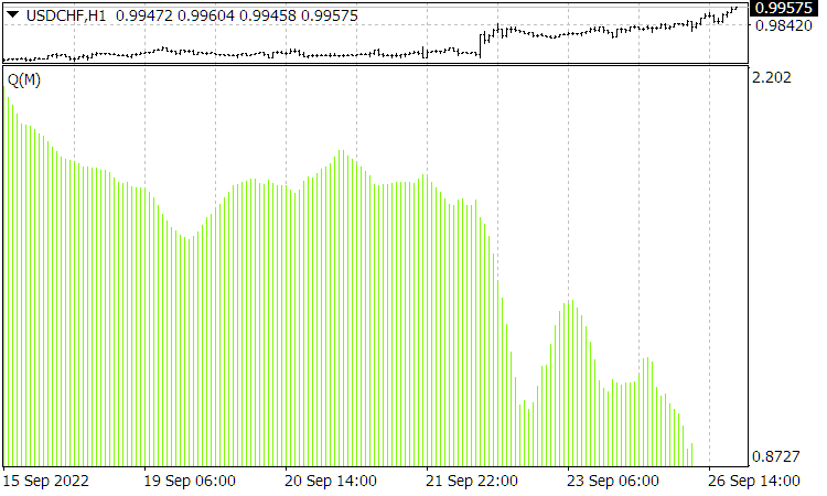
Fig. 4. Current ![]() function. The X axis here displays the averaging period for Quality Trend from 10 to 160, rather than time.
function. The X axis here displays the averaging period for Quality Trend from 10 to 160, rather than time.
Finally, the game is not based on an already formed history, but in real time, the knowledge of a number of forecasts ![]() , based on the
, based on the ![]() set of normalized velocity forecast values, is necessary. Therefore, to assess the possible length
set of normalized velocity forecast values, is necessary. Therefore, to assess the possible length ![]() of a newly emerging trend, we need to go through the entire spectrum of averaging periods and identify a number of maximums of the forecast quality
of a newly emerging trend, we need to go through the entire spectrum of averaging periods and identify a number of maximums of the forecast quality ![]() , when its forecasting goes forward by
, when its forecasting goes forward by ![]() bars from the current bar, i.e. calculated
bars from the current bar, i.e. calculated
 , (3.9)
where ![]() is an identification function of the
is an identification function of the ![]() th maximum. In this case, we also need to set the maximum peak
th maximum. In this case, we also need to set the maximum peak
 , (3.10)
and its corresponding point ![]() on the averaging scale.
on the averaging scale.
It is obvious that at smaller averaging intervals ![]() going to the maximum peak
going to the maximum peak ![]() of the forecast quality provided that at these intervals the quality is also significant and grows monotonically or in a sequence of increasing (also based on a growing backlog) peaks, there will be a corresponding unidirectional trend (with rollbacks after each peak of quality). After
of the forecast quality provided that at these intervals the quality is also significant and grows monotonically or in a sequence of increasing (also based on a growing backlog) peaks, there will be a corresponding unidirectional trend (with rollbacks after each peak of quality). After ![]() of the maximum peak
of the maximum peak ![]() of quality, when it begins to fall on the scale of the corresponding averaging
of quality, when it begins to fall on the scale of the corresponding averaging ![]() , there is a slowdown in the trend, which may soon lead to a reversal. The latter is most likely when the peak value
, there is a slowdown in the trend, which may soon lead to a reversal. The latter is most likely when the peak value ![]() is very significant in the sense that the quality factor for the exchange instrument under consideration rarely reaches values larger than
is very significant in the sense that the quality factor for the exchange instrument under consideration rarely reaches values larger than ![]() . In any case, the increasing trend will continue until the mark
. In any case, the increasing trend will continue until the mark ![]() , before reaching which we need to close the position opened according to this trend.
, before reaching which we need to close the position opened according to this trend.
Let us now try to estimate the lengths ![]() of trend segments that are promising for trading, which do not necessarily have to be equal to the predicted length of the
of trend segments that are promising for trading, which do not necessarily have to be equal to the predicted length of the ![]() trend. Firstly,, due to the low reliability of the work of predictive mathematics itself (which applies to all its types, even various frequency and other extrapolators, including neural networks and ARIMA, etc.), the profit should be taken on relatively small segments
trend. Firstly,, due to the low reliability of the work of predictive mathematics itself (which applies to all its types, even various frequency and other extrapolators, including neural networks and ARIMA, etc.), the profit should be taken on relatively small segments ![]() of the identified future trend
of the identified future trend ![]() , the trend is more likely to form on. Therefore, as follows from the previous paragraph, the
, the trend is more likely to form on. Therefore, as follows from the previous paragraph, the ![]() inequality should necessarily be fulfilled. Second, the presented model uses estimates of future probability values
inequality should necessarily be fulfilled. Second, the presented model uses estimates of future probability values ![]() and
and ![]() , as well as the average
, as well as the average ![]() leaps are assumed to be constant, since there are forecasts that work when the market develops by inertia and according to its own laws. However, as shown in the first article (Part 1), the interval of the predictable market development begins from the last strong external event and continues until the occurrence of the next such event. Therefore, there is the adequate work horizon
leaps are assumed to be constant, since there are forecasts that work when the market develops by inertia and according to its own laws. However, as shown in the first article (Part 1), the interval of the predictable market development begins from the last strong external event and continues until the occurrence of the next such event. Therefore, there is the adequate work horizon ![]() of the entire mathematical apparatus being developed here, where the quantity
of the entire mathematical apparatus being developed here, where the quantity ![]() is equal to the number of bars from the current bar to the future bar of the onset of a strong external event. If we try to use such a mathematical apparatus (which is extremely important) beyond a given horizon, this will cause errors in its operation and inevitable losses. To determine the possible horizon for the adequate operation of such a mathematical apparatus, it is necessary to build on fundamental analysis or expert research assessing the strength of influence of all current and future political and economic events on the state of the market. Therefore, the length of the forecast trend section promising for trading is estimated from above by the ratio
is equal to the number of bars from the current bar to the future bar of the onset of a strong external event. If we try to use such a mathematical apparatus (which is extremely important) beyond a given horizon, this will cause errors in its operation and inevitable losses. To determine the possible horizon for the adequate operation of such a mathematical apparatus, it is necessary to build on fundamental analysis or expert research assessing the strength of influence of all current and future political and economic events on the state of the market. Therefore, the length of the forecast trend section promising for trading is estimated from above by the ratio
![]() , (3.11)
, (3.11)
and from below it should be estimated on the basis of the previously established ratio of the smallness of the probability uncertainty (fluctuations) compared to the probability itself
![]() , (3.12)
, (3.12)
which is also determined from the predicted quality factor graph ![]() and corresponds to those areas where this graph changes quite smoothly. The expected natural price change in this section of the trend is
and corresponds to those areas where this graph changes quite smoothly. The expected natural price change in this section of the trend is
 , (3.13)
which corresponds to the order of profit obtained with a purely trend-following strategy.
Third, selection of the ![]() length of the trend segment should also be based on the calculations presented below, which essentially allows us to set the interval
length of the trend segment should also be based on the calculations presented below, which essentially allows us to set the interval ![]() values
values ![]() , on which it is possible to obtain an average statistical profit under given market conditions, i.e.
, on which it is possible to obtain an average statistical profit under given market conditions, i.e. ![]() . In addition to all this, traders chooses the timeframe on their own, and the true (and not the model, calculated by formula (3.8)) quality decreases with a decrease in the timeframe due to price noise on all timeframes by its non-model (identical on all timeframes) leaps. Therefore, traders are offered a choice of options with a high trend quality, but a long wait for profit, which is the case for large timeframes; or quickly making a profit on lower quality trends (and, accordingly, greater risks), which is typical for small timeframes.
. In addition to all this, traders chooses the timeframe on their own, and the true (and not the model, calculated by formula (3.8)) quality decreases with a decrease in the timeframe due to price noise on all timeframes by its non-model (identical on all timeframes) leaps. Therefore, traders are offered a choice of options with a high trend quality, but a long wait for profit, which is the case for large timeframes; or quickly making a profit on lower quality trends (and, accordingly, greater risks), which is typical for small timeframes.
4. Probabilistic calculation of the take profit and stop loss values that yield maximum profit at constant operating probabilities and the expression of the latter.
Setting a task.
The price moves in jumps in the vertical dimension from the zero mark. The probability of an upward price jump ![]() , the probability of a downward price jump
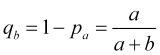
, the probability of a downward price jump ![]() , respectively,
, respectively, ![]() . Of course, there are predicted averages here
. Of course, there are predicted averages here ![]() and
and ![]() , which is not important now. At the top, there is the take profit at the distance of "a", while at the bottom, there is the stop loss at the distance of "в" from the zero mark (when viewed in the coordinate axes
, which is not important now. At the top, there is the take profit at the distance of "a", while at the bottom, there is the stop loss at the distance of "в" from the zero mark (when viewed in the coordinate axes ![]() ). Find the parameters of the stock exchange game that ensure maximum profit.
). Find the parameters of the stock exchange game that ensure maximum profit.
Solution.
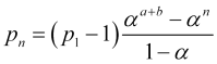
The price can go to the point with coordinate "n" or from below from the point "n-1" or from above from the point "n+1". Therefore, the probability of finding the price at point "n" is equal to
![]() . (4.1)
. (4.1)
From (4.1), we get the finite differences equation
![]() (4.2)
(4.2)
Equiprobable jumps.
Let us first consider the case of equiprobable jumps ![]() . Here we get the following from (4.2)
. Here we get the following from (4.2)
![]() , (4.3)
, (4.3)
where ![]() is a constant, from which we find
is a constant, from which we find
![]() . (4.4)
. (4.4)
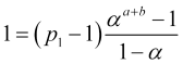
The probability of the price being at zero at the starting moment of its movement is ![]() , therefore,
, therefore,
![]() . (4.5)
. (4.5)
Let's assume that the stop loss "в" together with the take profit "a" constitute the characteristic (estimated here (3.4) in average price jumps ![]() ) price range
) price range ![]() of the movement over the
of the movement over the ![]() period of its averaging (and movement) the constancy of probabilities
period of its averaging (and movement) the constancy of probabilities ![]() and
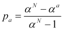
and ![]() is based on. The probability that the price is already at the stop loss point where
is based on. The probability that the price is already at the stop loss point where ![]() reaches a take profit reaches zero is
reaches a take profit reaches zero is ![]() . Substituting (4.5), we obtain
. Substituting (4.5), we obtain
 (4.6)
(4.6)
together with (4.5), this provides us with the probability of achieving take profit equal to
 (4.7)
(4.7)
while the probability of a stop loss being triggered
 . (4.8)
Therefore, with equally probable price jumps in different directions, the average profit in the number of jumps
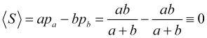 (4.9)
(4.9)
is always zero (the spread, of course, makes it negative) regardless of the position of the take profit and stop loss, which can be anything.
There is a tendency to move towards take profit .
Let ![]() (or, to be more accurate,
(or, to be more accurate, ![]() ) then, multiplying all equations (4.2), we find
) then, multiplying all equations (4.2), we find
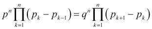 , (4.10)
reducing identical factors in (4.10), using notation (2.7) ![]() and considering that
and considering that ![]() , we obtain
, we obtain
![]() . (4.11)
. (4.11)
Let's display ![]() as the sum of the differences of adjacent terms of the probability series
as the sum of the differences of adjacent terms of the probability series ![]() using further relations (4.11) and the equation for summing the geometric progression
using further relations (4.11) and the equation for summing the geometric progression
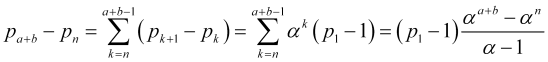 , (4.12)
![]() , therefore,
, therefore,
 (4.13)
![]() , hence,
, hence,
 , (4.14)
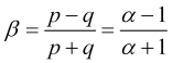
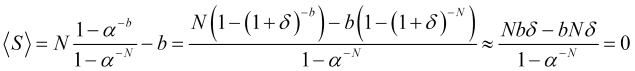
dividing (4.13) by (4.14), we obtain the probability of achieving take profit "а"
 . (4.15)
The probability of the stop loss being triggered is, accordingly, equal to ![]() . Then the average profit per one position in price jumps
. Then the average profit per one position in price jumps ![]() is equal to
is equal to
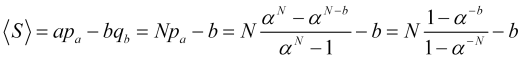 , (4.16)
which in the representation (4.16) is a function of the stop loss value "в", which in this representation is simply a number of ![]() jumps, but in fact there is a value of
jumps, but in fact there is a value of ![]() . The profit is
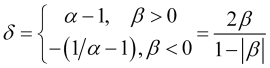
. The profit is ![]() . It is clear that with an increase in the probability of price movement towards an open position, the average profit (4.16) increases. When
. It is clear that with an increase in the probability of price movement towards an open position, the average profit (4.16) increases. When ![]() takes the value of
takes the value of ![]() , i.e.
, i.e. ![]() is a growing function from
is a growing function from ![]() .
.
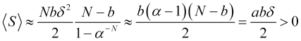
Let's find the maximum of the average statistical profit (4.16) subject to the given values of N and ![]() . To achieve this, let's equate its derivative to zero
. To achieve this, let's equate its derivative to zero
 , (4.17)
from where we find the value of the desired stop loss in ![]() price leaps
price leaps
 . (4.18)
Since ![]() , the
, the ![]() logarithm is positive and
logarithm is positive and ![]() . Accordingly, the logarithm
. Accordingly, the logarithm  value should be positive. This condition is satisfied if
![]() , (4.19)
, (4.19)
or
![]() , (4.20)
, (4.20)
where ![]() . The (4.20) inequality is strictly satisfied for any
. The (4.20) inequality is strictly satisfied for any ![]() , since the
, since the ![]() exponent passes above the straight line
exponent passes above the straight line ![]() touching it only at
touching it only at ![]() .
.
The second derivative of the function (4.16)
 (4.21)
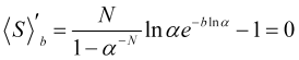
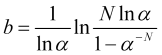
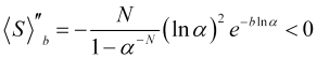
is always negative under these conditions, i.e. the curvature of the ![]() function is directed downward and we have the maximum at (4.18). The function (4.16) at N=100 and
function is directed downward and we have the maximum at (4.18). The function (4.16) at N=100 and ![]() is displayed in Fig. 5.
is displayed in Fig. 5.
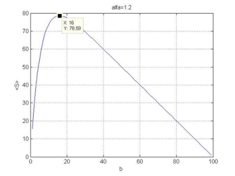
Fig.5. Dependence of the profit function on stop loss.
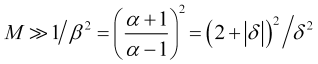
Keep in mind that in order for the average profit ![]() to be positive, the
to be positive, the ![]() ratio should significantly exceed one. Indded, if
ratio should significantly exceed one. Indded, if ![]() , where
, where ![]() and we can neglect the second term of the expansion, leaving only the first term
and we can neglect the second term of the expansion, leaving only the first term ![]() , then the average profit per trade
, then the average profit per trade
 (4.22)
will be equal to zero (as in the case of equal probabilities of opposite jumps). If the second term of the expansion cannot be neglected, then taking into account that the number of jumps ![]() is big enough or
is big enough or ![]() , we have
, we have
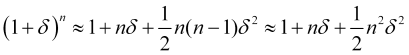 , (4.23)
which will give a positive value for the average profit (4.16)
 , (4.24)
since ![]() ,
, ![]() (and, therefore,
(and, therefore, ![]() ).
).
The approximate average profit (4.24) relative to the argument ![]() is an inverted quadratic parabola whose maximum is reached at
is an inverted quadratic parabola whose maximum is reached at ![]() (which is the equality of stop loss and take profit), when
(which is the equality of stop loss and take profit), when ![]() .
.
Here is a very important point. In the theory presented above, the average profit was calculated only on the basis of average price values, which, in fact, fluctuates greatly and can even greatly exceed the corresponding average shifts in the range of its fluctuations. However, stop orders (take profit and stop loss) are closed not at the average price values, but precisely at the edges of the band of its fluctuations. Therefore, in order for the presented mathematical apparatus (based on average values) to work, the stop loss should greatly exceed ![]() the price uncertainty
the price uncertainty ![]() (so that its fluctuation triggering differs little from the model triggering in terms of the average and these fluctuations can be neglected), i.e., according to (1.2),
(so that its fluctuation triggering differs little from the model triggering in terms of the average and these fluctuations can be neglected), i.e., according to (1.2),
![]() . (4.25)
. (4.25)
In this case, using the (3.7.1) expressions for the averaging period, get from (4.25) the function the following inequality should be satisfied for
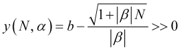 , (4.26)
which is a criterion for the smallness of price fluctuations, where ![]() is found from the (2.6) ratio. By substituting into (4.26) the (4.18) stop loss, we get the function graph (Fig. 6), which makes clear that such a function is not much greater than zero, but, on the contrary, is fundamentally negative, i.e. the ratio (4.25) is never satisfied with the optimal stop loss (4.18).
is found from the (2.6) ratio. By substituting into (4.26) the (4.18) stop loss, we get the function graph (Fig. 6), which makes clear that such a function is not much greater than zero, but, on the contrary, is fundamentally negative, i.e. the ratio (4.25) is never satisfied with the optimal stop loss (4.18).
MATLAB code
>> [N,a]=meshgrid([3:200],[1.01:0.01:3]);
>> b=log(N.*log(a)./(1-a.^(-N)))./log(a);
>> beta=(a-1)./(a+1);
>> s=(N.*beta+1).^(1/2)./beta;
>> y=b-s;
>> plot3(N,a,y)
>> grid on
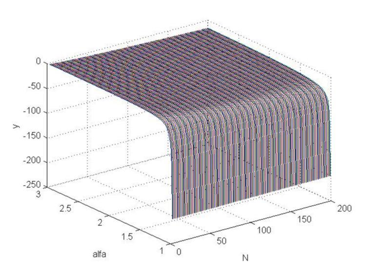
Fig.6. "y" function graph when changing Alpha from 1 to 3 and changing N from 3 to 200.
Thus, the use of the stop order values calculated above will lead to average statistical losses, since price fluctuations turn out to be fundamentally greater than the optimal one in the model of its average stop loss movement
![]() . (4.27)
. (4.27)
This means we need to change the size of the stop loss itself, rather than look for the averaging period which makes the optimal stop loss (4.18) relatively small (4.25) (since this task has no solution). This will, of course, change the profit as well.
The optimal take profit for the average price movement model coincides with the point of the forecast moving average price, which is located ![]() bars ahead of the current bar. But if we take into account strong price deviations from the average, at which stop orders are closed, then (as can be seen in the Casual Channel indicator graph in Fig. 1), to ensure a profitable game, such an optimal take profit should be reduced by an amount greater than the average deviation
bars ahead of the current bar. But if we take into account strong price deviations from the average, at which stop orders are closed, then (as can be seen in the Casual Channel indicator graph in Fig. 1), to ensure a profitable game, such an optimal take profit should be reduced by an amount greater than the average deviation
![]() , (4.28)
, (4.28)
where the ![]() ratio should be slightly greater than one for weak trends (having almost no profit) and approximately
ratio should be slightly greater than one for weak trends (having almost no profit) and approximately ![]() for strong trends, being here exactly the parameter whose exact value should be sought through optimization, and the stop loss should be increased by the same amount, i.e.
for strong trends, being here exactly the parameter whose exact value should be sought through optimization, and the stop loss should be increased by the same amount, i.e.
![]() . (4.29)
. (4.29)
Then, a stop loss, as a value separated from the average value of the possible price deviation (for ![]() future bars) against an open position by
future bars) against an open position by ![]() , will be triggered much less often with a probability lower than
, will be triggered much less often with a probability lower than ![]() , while take profit will be triggered more often with a greater probability exceeding
, while take profit will be triggered more often with a greater probability exceeding ![]() . Accordingly, for the maximum profit, we obtain the estimate
. Accordingly, for the maximum profit, we obtain the estimate
![]() , (4.30)
, (4.30)
where ![]() is a value from (4.16), or considering (3.7.1)
is a value from (4.16), or considering (3.7.1)
 (4.31)
whose function (in case of the optimal b from (4.18)) can be constructed, so that we are able to find the N value maximizing it, as well as the averaging period.
MATLAB code for k=3
>> [N,a]=meshgrid([3:200],[1.01:0.01:3]);
>> b=log(N.*log(a)./(1-a.^(-N)))./log(a);
>> beta=(a-1)./(a+1);
>> s=(N.*beta+1).^(1/2)./beta;
>> s0=N.*(1-a.^(-b))./(1-a.^(-N))-b;
>> Profit=s0-3*s;
>> plot3(N , a, Profit)
>> grid on
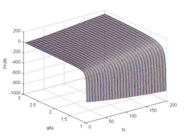
Fig.7. Profit function graph (in model price jumps) as Alpha changes from 1 to 3 and N from 3 to 200.
The graph shows that the profit with a positive mathematical expectation is generally possible and increases with increasing Alpha and N.
To find the most promising averaging period ![]() , we need to construct a predictive quality factor function
, we need to construct a predictive quality factor function ![]() . This is why the CalculateScientificTradePeriod script has been developed. We need to define the most promising period
. This is why the CalculateScientificTradePeriod script has been developed. We need to define the most promising period ![]() by the
by the ![]() maximum location where
maximum location where ![]() when this maximum is reached smoothly (the (3.12) ratio is fulfilled) and is not located further than the adequate work horizon. If the
when this maximum is reached smoothly (the (3.12) ratio is fulfilled) and is not located further than the adequate work horizon. If the ![]() value found in this way provides a positive (as well as exceeding at least a couple of spreads) profit value (4.31) and a sufficiently high probability of winning (4.15), which sets the interval
value found in this way provides a positive (as well as exceeding at least a couple of spreads) profit value (4.31) and a sufficiently high probability of winning (4.15), which sets the interval ![]() , then the trading decision should be based on it here. In order to calculate the optimal (maximizing the average profit) take profit and stop loss, as well as to determine the further price trend, I have developed the ScientificTrade indicator, whose algorithms are based on the entire theory presented above.
, then the trading decision should be based on it here. In order to calculate the optimal (maximizing the average profit) take profit and stop loss, as well as to determine the further price trend, I have developed the ScientificTrade indicator, whose algorithms are based on the entire theory presented above.
Note that the CalculateScientificTradePeriod script algorithm is very resource-intensive, so we use the script, not the indicator, which would run this algorithm on every tick and would freeze the computer. The FindScientificTradePeriod indicator is used to display data calculated by the script.
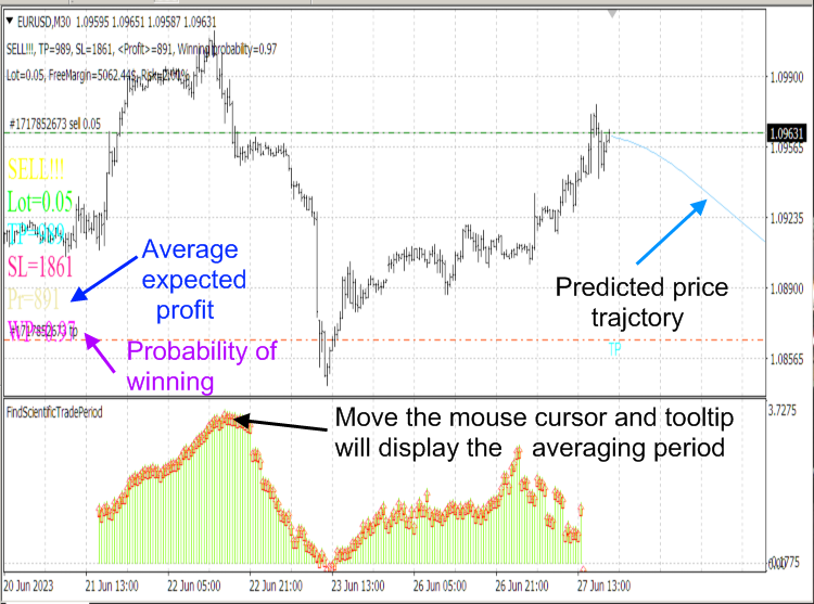
Fig. 8. ScientificTrade and FindScientificTradePeriod indicators.
Fig. 9. ScientificTrade indicator results.
5. Irremovable error of applied calculations within the framework of the mathematical apparatus itself. The approach to identifying moments of naturally occurring price rebounds and reversals.
As was previously said, the trends predicted by the ScientificTrade indicator and calculated by the stop loss and take profit location indicator are based on the ![]() and
and ![]() forecast values, which may turn out to be erroneous due to the unreliability of the forecasting apparatus itself (in the Fourier extrapolator indicator). Therefore, such forecasts may turn out to be false within the adequate work horizon of all the mathematical apparatus presented above.
forecast values, which may turn out to be erroneous due to the unreliability of the forecasting apparatus itself (in the Fourier extrapolator indicator). Therefore, such forecasts may turn out to be false within the adequate work horizon of all the mathematical apparatus presented above.
To exclude at least some cases of false mathematical forecasts, trends calculated by the ScientificTrade indicator on the interval determined by the CalculateScientificTradePeriod script, should coincide with the forecast trends provided by authoritative fundamental analysis experts for a given interval. It is clear that if both ScientificTrade and the experts provide the same false forecast (which we cannot know about), then losses are also inevitable. According to my subjective observations, experts are more likely to make mistakes than the ScientificTrade indicator in combination with the CalculateScientificTradePeriod script, which, in my opinion, is due to the fact that inner laws of market development have a stronger impact than most external events causing changes in trends experts are not able to determine. Moreover, such market reversals caused by internal reasons often occur before the onset of strong external events, as well as more often than those events. The appropriate mechanisms will be discussed below.
To express the essence of the above problem, it should first be noted that the price, does not always move in equidistant jumps even when the market develops according to its own laws (when the price is not pushed by strong external events). This concept is a simplified model, which allows us to understand at least something and make calculations in the market chaos. In reality, the price occasionally makes short-term (beyond the scope of classical statistics) strong movements contrary to average static trends, according to which it slowly drifts (with large fluctuations) in a certain direction. Moreover, if such strong movements are not caused by external influences on the market, but originate from its inner processes, then they are usually directed against statistical trends. Therefore, such strong movements knock down stop losses and create maximum losses for most small traders.
In fact (if we exclude the purposeful knocking down of stop losses by providers of trading services and quotes), Le Chatelier’s principle works here in conjunction with the dialectical law of the transition of quantity into quality. Upon reaching a specific (also dependent on the market) growth (or fall) level of a certain market instrument, a sharp jump in quality occurs, which, in accordance with Le Chatelier’s principle (the action of which extends to any complex system in equilibrium, including the economy, which most of the time evolves passing through close quasi-equilibrium states), tends to resist the growth of the above-mentioned quantity sharply lowering it (in a jump). Since the market as a system, with its monotonous development, gradually passes through close quasi-equilibrium states, Le Chatelier’s principle does not react to its small changes, but acts abruptly when large quantitative changes are already accumulating in a given system. From the standpoint of the market wave model (Part 1), such jumps can be explained by the advancing proximity (or equality) of the phases of partial probability waves of the corresponding market instrument.
Theoretically, the approach of a natural price jump can be identified using the ratio (II.17). However, in practice, it is much easier to detect an approaching jump using the predicted quality factor graph. In particular, if the predicted quality factor at some future moment ![]() (distant from the current bar by
(distant from the current bar by ![]() bars) exceeds or approaches a certain critical value for a given market instrument on the corresponding timeframe
bars) exceeds or approaches a certain critical value for a given market instrument on the corresponding timeframe ![]() , i.e.
, i.e. ![]() (if we consider the current and not the forecast situation, then simply
(if we consider the current and not the forecast situation, then simply ![]() ), then at this moment a change in the global trend is possible.
), then at this moment a change in the global trend is possible.
In general, natural price jumps (of any nature, both global and small) at the level of probability amplitudes of its distribution are described by antisymmetric wavelets (Part 1, ratio (I.17)), when, after realizing the proximity and even equality of the phases of all partial price waves, from which its total probability amplitude is composed, the phase of the latter, due to the antisymmetry of the corresponding wavelets, is inverted, which leads to a sharp change in the actual ![]() and
and ![]() probabilities, which will then be fundamentally different from the forecast probabilities
probabilities, which will then be fundamentally different from the forecast probabilities ![]() and
and ![]() . It is clear that such critical situations, when jumps in quality occur due to the market’s own laws, should be excluded from trading. Such antisymmetry of partial price waves ensures their similarity to fermions, which determines the constant desire to change price levels and their significant width (which is interpreted as a result of price fluctuations). Therefore, it is more correct to describe the evolution of market instruments not by ordinary statistics, but by Fermi-Dirac statistics.
. It is clear that such critical situations, when jumps in quality occur due to the market’s own laws, should be excluded from trading. Such antisymmetry of partial price waves ensures their similarity to fermions, which determines the constant desire to change price levels and their significant width (which is interpreted as a result of price fluctuations). Therefore, it is more correct to describe the evolution of market instruments not by ordinary statistics, but by Fermi-Dirac statistics.
Due to the described effect of price wave inversion (Part 1) at the most intense phase of its movement (the maximum modulus of the amplitude of its probability), it is also funny to note that, it would seem, the most optimal trading parameters based on the highest ![]() quality factor should also ensure maximum profit. However, these trading parameters identified by most traders (intuitively or mathematically) on the basis of habitual ideas (characteristic of everything observed in the physical macrocosm) about the monotony of processes and their inertia, in fact, cause maximum losses.
quality factor should also ensure maximum profit. However, these trading parameters identified by most traders (intuitively or mathematically) on the basis of habitual ideas (characteristic of everything observed in the physical macrocosm) about the monotony of processes and their inertia, in fact, cause maximum losses.
As a result, the everyday "law" turns out to be true here too: money begets money, the bulk of which is stored in banks, so the market pulls money out of small traders. After all, the market, for the reasons mentioned above, suddenly (which it does regularly) begins to develop contrary to the trends predicted by the majority of traders playing against them. This process has no human "evil" intent. The market does not have constant inertia (used by small traders to get profit for some period of time) characteristic of physical macro processes and, at certain moments (unpredictable for experts and traders not armed with the appropriate theory), it easily reverses the phases of all individual partial price waves emitted by different market participants under the influence of its inner laws operating at its emergent level (surpassing the influence of even strong external events).
Overall, the market is ruled by chaos. That's why, if any market order is identified to the maximum extent, then it must be violated, which can be considered a fairly well-observed law of the market. It is impossible to obtain a stable profit without knowing it.
Conclusion
The article presents my engineering approach to creating a profitable trading strategy. This approach shows that the market leaves traders an extremely narrow set of conditions for opening and closing positions, which could provide them with a game with a positive expected profit. This set is not identifiable by classical methods. But a game with a positive profit expectation is still possible, which to some extent is confirmed by my personal use of the ScientificTrade indicator based on this engineering approach and the use of Fourier extrapolation for prediction (although the statistics is far from sufficient so far). Of course, this indicator still needs to be improved. At the moment, its main drawback is the use of an insufficiently accurate mathematical forecasting apparatus.
Translated from Russian by MetaQuotes Ltd.
Original article: https://www.mql5.com/ru/articles/12891
Warning: All rights to these materials are reserved by MetaQuotes Ltd. Copying or reprinting of these materials in whole or in part is prohibited.
This article was written by a user of the site and reflects their personal views. MetaQuotes Ltd is not responsible for the accuracy of the information presented, nor for any consequences resulting from the use of the solutions, strategies or recommendations described.

- Free trading apps
- Over 8,000 signals for copying
- Economic news for exploring financial markets
You agree to website policy and terms of use