
Data Science and Machine Learning (Part 15): SVM, A Must-Have Tool in Every Trader's Toolbox

Contents:
- Introduction
- What is a hyperplane?
- Linear SVM
- Dual SVM
- Hard Margin
- Soft Margin
- Training a Linear Support Vector Machine Model
- Getting Predictions from Linear Support Vector Model
- Train Test the Linear SVM model
- Collecting and Normalizing Data
- DualSVMONNX class instance | Initializing a class
- Training the Dual SVM model in python
- Converting SVC model sklearn to ONNX and saving
- Final Thoughts
Introduction
Support Vector Machine (SVM) is a powerful supervised machine learning algorithm used for linear or nonlinear classification and regression tasks, and sometimes outlier detection tasks.
Unlike Bayesian classification techniques, and logistic regression which deploy simple mathematical models to classify information, The SVM has some complex mathematical learning functions aimed at finding the optimal hyperplane that separates the data in an N-dimensional space.
Support vector machine is usually used for classification tasks, something we'll also do in this article
What is a hyperplane?
A hyperplane is a line used to separate data points of different classes.

The hyperplane has the following properties:
Dimensionality: In a binary classification problem, the hyperplane is a (d-1)-dimensional subspace, where "d" is the dimension of the feature space. For example, in a two-dimensional feature space, the hyperplane is a one-dimensional line.
Equation: Mathematically, a hyperplane can be represented by a linear equation of the form:
![]()
![]() is a vector that is orthogonal to the hyperplane and determines its orientation.
is a vector that is orthogonal to the hyperplane and determines its orientation.
![]() is a feature vector.
is a feature vector.
b is a scalar bias term that shifts the hyperplane away from the origin.
Separation: The hyperplane divides the feature space into two half-spaces:
The region where ![]() corresponds to one class.
corresponds to one class.
The region where ![]() corresponds to the other class.
corresponds to the other class.
Margin: In SVM, the goal is to find the hyperplane that maximizes the margin, which is the distance between the hyperplane and the nearest data points from either class. These nearest data points are called "support vectors." The SVM aims to find the hyperplane that achieves the maximum margin while minimizing the classification error.
Classification: Once the optimal hyperplane is found, it can be used to classify new data points. By evaluating ![]() , you can determine on which side of the hyperplane a data point falls, and thus classify it into one of the two classes.
, you can determine on which side of the hyperplane a data point falls, and thus classify it into one of the two classes.
The concept of a hyperplane is a key element in SVM because it forms the basis for the maximum-margin classifier. SVMs aim to find the hyperplane that best separates the data while maintaining a maximum margin between classes, which, in turn, enhances the model's generalization and robustness to unseen data.
double CLinearSVM::hyperplane(vector &x)
 {
   return x.MatMul(W) - B;
 }
As said earlier the bias term denoted as b is a scalar term so a double variable had to be declared for it.
class CLinearSVM
  {
   protected:

      CMatrixutils      matrix_utils;
      CMetrics          metrics;

      CPreprocessing<vector, matrix> *normalize_x;

      vector            W; //Weights vector
      double            B; //bias term

      bool is_fitted_already;

      struct svm_config
        {
          uint batch_size;
          double alpha;
          double lambda;
          uint epochs;
        };

   private:
      svm_config config;
We have seen the class name CLinearSVM that explains for itself that this is a linear Support vector Machine, this brings us to the aspects of SVM, where we have Linear and Dual Support Vector Machine
Linear SVM
A linear SVM is a type of SVM that employs a linear kernel, which means it uses a linear decision boundary to separate data points. In a linear SVM, you are working directly with the feature space, and the optimization problem is often expressed in its primal form. The primary goal of a linear SVM is to find a linear hyperplane that best separates the data.
This works best for linear separable data.
Dual SVM
The dual SVM is not a distinct type of SVM but rather a representation of the SVM optimization problem. The dual form of an SVM is a mathematical reformulation of the original optimization problem that allows for more efficient solution methods. It introduces Lagrange multipliers to maximize a dual objective function, which is equivalent to the primal problem. Solving the dual problem leads to the determination of support vectors, which are critical for classification.
This best suits the data that is not linearly separable

It is also important to know that we can either use hard or soft margins to make SVM classifier decisions using hyperplane.
Hard Margin
if the training data is linearly separable, we can select two parallel hyperplanes that separate the two classes of data, so that the distance between them is as large as possible. The region bounded by these two hyperplanes is called the "margin", and the maximum-margin hyperplane is the hyperplane that lies halfway between them. With a normalized or standardized dataset, these hyperplanes can be described by the equations
![]() (anything on or above this boundary is of one class, with label 1)
(anything on or above this boundary is of one class, with label 1)
and
![]() (anything on or below this boundary is of the other class, with label −1).
(anything on or below this boundary is of the other class, with label −1).
The distance between them is 2/||w|| and to maximize the distance, ||w|| should be minimum. To prevent any data point falling inside margin we add the restriction, yi(wTXi -b) >= 1 where yi = ith row in the target and Xi = ith row in the X
Soft Margin
To extend SVM to cases in which the data are not linearly separable, the hinge loss function is helpful
![]() .
.
Note that ![]() is the i-th target (i.e., in this case, 1 or −1), and
is the i-th target (i.e., in this case, 1 or −1), and ![]() is the i-th output.
is the i-th output.
If the data point has class = 1, then the loss will be 0, otherwise it will be the distance between the margin and the data point. and our goal is to minimize
![]() where λ is a tradeoff between the margin size and xi being on the correct side of margin. If λ is too low, the equation becomes hard margin.
where λ is a tradeoff between the margin size and xi being on the correct side of margin. If λ is too low, the equation becomes hard margin.
We'll be using the hard margin, for the Linear SVM class, this is made possible by the sign function, which is a function that returns the sign of a real number in mathematical notation. Expressed as:
int CLinearSVM::sign(double var)
 {
   if (var == 0)
    return (0);
   else if (var < 0)
    return -1;
   else
    return 1;
 }
Training a Linear Support Vector Machine Model
The training process of a Support Vector Machine (SVM) involves finding the optimal hyperplane that separates the data while maximizing the margin. The margin is the distance between the hyperplane and the nearest data points from either class. The goal is to find the hyperplane that maximizes the margin while minimizing classification errors.
Updating Weights (w):
a. First Term: The first term in the loss function corresponds to the hinge loss, which measures the classification error. For each training example i, we compute the derivative of the loss with respect to the weights w as follows:
- If
 , which means the data point is correctly classified and outside the margin, the derivative is 0.
 - If
 , which means the data point is inside the margin or misclassified, the derivative is
  .
.
b. Second Term:
The second term represents the regularization term. It encourages a small margin and helps prevent overfitting. The derivative of this term with respect to the weights w is 2λw, where λ is the regularization parameter.
c. Combining the derivatives of the first and second terms,
The update for the weights w is as follows:
-If ![]() , we update the weights as follows:
, we update the weights as follows: ![]() if
if ![]() , we update the weights as follows:
, we update the weights as follows: ![]() Here, α is the learning rate.
Here, α is the learning rate.
Updating Intercept (b):
a. First Term:
The derivative of the hinge loss with respect to the intercept b is computed similarly to the weights:
- If
 , the derivative is 0.
 - If
 , the derivative is
  .
.
b. Second Term:
The second term does not depend on the intercept, so its derivative with respect to b is 0. c. The update for the intercept b is as follows:
- If
 , we update
  as follows:
- If
 , we update
  as follows:
Slack Variable (ξ):
The slack variable (ξ) allows for some data points to be inside the margin, which means they are misclassified or within the margin. The condition ![]() represents that the decision boundary should be at least
represents that the decision boundary should be at least ![]() units away from data point i.
units away from data point i.
In summary, the training process of an SVM involves updating the weights and intercept based on the hinge loss and the regularization term. The objective is to find the optimal hyperplane that maximizes the margin while considering potential misclassifications inside the margin allowed by the slack variable. This process is typically solved using optimization techniques, and support vectors are identified during the training process to define the decision boundary.
void CLinearSVM::fit(matrix &x, vector &y)
 {
   matrix X = x;
   vector Y = y;

   ulong rows = X.Rows(),
         cols = X.Cols();

   if (X.Rows() != Y.Size())
      {
         Print("Support vector machine Failed | FATAL | X m_rows not same as yvector size");
         return;
      }

   W.Resize(cols);
   B = 0;

   normalize_x = new CPreprocessing<vector, matrix>(X, NORM_STANDARDIZATION); //Normalizing independent variables

//---

  if (rows < config.batch_size)
    {
      Print("The number of samples/rows in the dataset should be less than the batch size");
      return;
    }

    matrix temp_x;
    vector temp_y;
    matrix w, b;

    vector preds = {};
    vector loss(config.epochs);
    during_training = true;

    for (uint epoch=0; epoch<config.epochs; epoch++)
      {

         for (uint batch=0; batch<=(uint)MathFloor(rows/config.batch_size); batch+=config.batch_size)
           {
              temp_x = matrix_utils.Get(X, batch, (config.batch_size+batch)-1);
              temp_y = matrix_utils.Get(Y, batch, (config.batch_size+batch)-1);

              #ifdef DEBUG_MODE:
                  Print("X\n",temp_x,"\ny\n",temp_y);
              #endif

               for (uint sample=0; sample<temp_x.Rows(); sample++)
                  {
                     // yixiw-b≥1

                      if (temp_y[sample] * hyperplane(temp_x.Row(sample))  >= 1)
                        {
                          this.W -= config.alpha * (2 * config.lambda * this.W); // w = w + α* (2λw - yixi)
                        }
                      else
                         {
                           this.W -= config.alpha * (2 * config.lambda * this.W - ( temp_x.Row(sample) * temp_y[sample] )); // w = w + α* (2λw - yixi)

                           this.B -= config.alpha * temp_y[sample]; // b = b - α* (yi)
                         }
                  }
           }

        //--- Print the loss at the end of an epoch

         is_fitted_already = true;

         preds = this.predict(X);

         loss[epoch] = preds.Loss(Y, LOSS_BCE);

         printf("---> epoch [%d/%d] Loss = %f Accuracy = %f",epoch+1,config.epochs,loss[epoch],metrics.confusion_matrix(Y, preds, false));

        #ifdef DEBUG_MODE:
          Print("W\n",W," B = ",B);
        #endif
      }

    during_training = false;

    return;
 }
Getting Predictions from Linear Support Vector Model
To get the predictions out of the model data must be passed to the sign function after the hyperplane has given an output.
int CLinearSVM::predict(vector &x)
 {
   if (!is_fitted_already)
     {
       Print("Err | The model is not trained, call the fit method to train the model before you can use it");
       return 1000;
     }

   vector temp_x = x;
   if (!during_training)
     normalize_x.Normalization(temp_x); //Normalize a new input data when we are not running the model in training

   return sign(hyperplane(temp_x));
 }
Train Test the Linear SVM model
As a common practice, it is good to test the model before we can deploy it to make any significant predictions on market data, let us start by initializing the Linear SVM class instance.
#include <MALE5\Support Vector Machine(SVM)\svm.mqh>
CLinearSVM *svm;

input uint bars = 1000;
input uint epochs_ = 1000;
input uint batch_size_ = 64;
input double alpha__ =0.1;
input double lambda_ = 0.01;

bool train_once;
//+------------------------------------------------------------------+
//| Expert initialization function                                   |
//+------------------------------------------------------------------+
int OnInit()
  {
//---
    svm = new CLinearSVM(batch_size_, alpha__, epochs_, lambda_);
    train_once = false;
//---

   return(INIT_SUCCEEDED);
  }
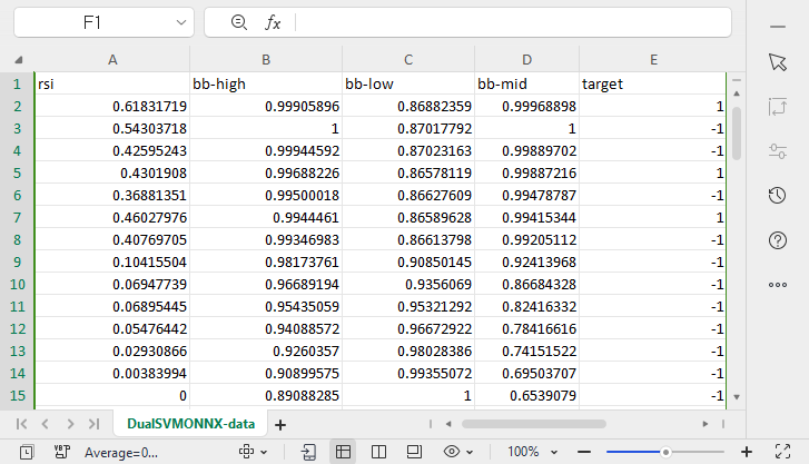
We'll proceed collecting the data, We'll be using the 4 independent variables which are RSI, BOLLINGER BANDS HIGH, LOW and MID.
vec_.CopyIndicatorBuffer(rsi_handle, 0, 0, bars);
dataset.Col(vec_, 0);
vec_.CopyIndicatorBuffer(bb_handle, 0, 0, bars);
dataset.Col(vec_, 1);
vec_.CopyIndicatorBuffer(bb_handle, 1, 0, bars);
dataset.Col(vec_, 2);
vec_.CopyIndicatorBuffer(bb_handle, 2, 0, bars);
dataset.Col(vec_, 3);

open.CopyRates(Symbol(), PERIOD_CURRENT, COPY_RATES_OPEN, 0, bars);
close.CopyRates(Symbol(), PERIOD_CURRENT, COPY_RATES_CLOSE, 0, bars);

for (ulong i=0; i<vec_.Size(); i++) //preparing the independent variable
   dataset[i][4] = close[i] > open[i] ? 1 : -1; // if price closed above its opening thats bullish else bearish
We finish the data collection process by splitting the data into training and testing samples.
matrix_utils.TrainTestSplitMatrices(dataset,train_x,train_y,test_x,test_y,0.7,42); //split the data into training and testing samples
Training/ Fitting the Model
svm.fit(train_x, train_y);
Outputs:
        0       15:15:42.394    svm test (EURUSD,H1)    ---> epoch [1/1000] Loss = 7.539322 Accuracy = 0.489000
IK      0       15:15:42.395    svm test (EURUSD,H1)    ---> epoch [2/1000] Loss = 7.499849 Accuracy = 0.491000
EG      0       15:15:42.395    svm test (EURUSD,H1)    ---> epoch [3/1000] Loss = 7.499849 Accuracy = 0.494000
....
....
GG      0       15:15:42.537    svm test (EURUSD,H1)    ---> epoch [998/1000] Loss = 6.907756 Accuracy = 0.523000
DS      0       15:15:42.537    svm test (EURUSD,H1)    ---> epoch [999/1000] Loss = 7.006438 Accuracy = 0.521000
IM      0       15:15:42.537    svm test (EURUSD,H1)    ---> epoch [1000/1000] Loss = 6.769601 Accuracy = 0.516000
Observing the accuracy of the model in both training and testing.
vector train_pred = svm.predict(train_x),
    test_pred = svm.predict(test_x);

printf("Train accuracy = %f",metrics.confusion_matrix(train_y, train_pred, true));
printf("Test accuracy = %f ",metrics.confusion_matrix(test_y, test_pred, true));
Outputs:
CH      0       15:15:42.538    svm test (EURUSD,H1)    Confusion Matrix
IQ      0       15:15:42.538    svm test (EURUSD,H1)    [[171,175]
HE      0       15:15:42.538    svm test (EURUSD,H1)     [164,190]]
DQ      0       15:15:42.538    svm test (EURUSD,H1)
NO      0       15:15:42.538    svm test (EURUSD,H1)    Classification Report
JD      0       15:15:42.538    svm test (EURUSD,H1)
LO      0       15:15:42.538    svm test (EURUSD,H1)    _    Precision  Recall  Specificity  F1 score  Support
JQ      0       15:15:42.538    svm test (EURUSD,H1)    -1.0    0.51     0.49     0.54       0.50     346.0
DH      0       15:15:42.538    svm test (EURUSD,H1)    1.0    0.52     0.54     0.49       0.53     354.0
HL      0       15:15:42.538    svm test (EURUSD,H1)
FG      0       15:15:42.538    svm test (EURUSD,H1)    Accuracy                                   0.52
PP      0       15:15:42.538    svm test (EURUSD,H1)    Average   0.52    0.52    0.52      0.52    700.0
PS      0       15:15:42.538    svm test (EURUSD,H1)    W Avg     0.52    0.52    0.52      0.52    700.0
FK      0       15:15:42.538    svm test (EURUSD,H1)    Train accuracy = 0.516000

MS      0       15:15:42.538    svm test (EURUSD,H1)    Confusion Matrix
LI      0       15:15:42.538    svm test (EURUSD,H1)    [[79,74]
CM      0       15:15:42.538    svm test (EURUSD,H1)     [68,79]]
FJ      0       15:15:42.538    svm test (EURUSD,H1)
HF      0       15:15:42.538    svm test (EURUSD,H1)    Classification Report
DM      0       15:15:42.538    svm test (EURUSD,H1)
NH      0       15:15:42.538    svm test (EURUSD,H1)    _    Precision  Recall  Specificity  F1 score  Support
NN      0       15:15:42.538    svm test (EURUSD,H1)    -1.0    0.54     0.52     0.54       0.53     153.0
PQ      0       15:15:42.538    svm test (EURUSD,H1)    1.0    0.52     0.54     0.52       0.53     147.0
JE      0       15:15:42.538    svm test (EURUSD,H1)
GP      0       15:15:42.538    svm test (EURUSD,H1)    Accuracy                                   0.53
RI      0       15:15:42.538    svm test (EURUSD,H1)    Average   0.53    0.53    0.53      0.53    300.0
JH      0       15:15:42.538    svm test (EURUSD,H1)    W Avg     0.53    0.53    0.53      0.53    300.0
DO      0       15:15:42.538    svm test (EURUSD,H1)    Test accuracy = 0.527000
Our model was 53% accurate in out-of-sample predictions, some would say a bad model, but I would say an average model. There might be many factors leading to this including bugs in the model, poor normalization, convergence criteria, and much more, you can try adjusting the parameters to see what leads to a better outcome. However, it could also be that the data is too complex for a linear model, about that I'm confident so let's try dual SVM to see if it helps.
For the dual SVM we are going to explore in ONXX python format, I wasn't able to get the mql5 coded model to get close to the python sklearn dual SVM model performance and accuracy wise so I think it's worth exploring dual SVM in python for now, The dual SVM library in MQL5 can still be found the main svm.mqh file provided in this article and on my GitHub linked at the end of this article.
To kick start dual SVM in Python we need to collect data and Normalize using mql5, We might need to create a new class with the name CDualSVMONNX inside svm.mqh file, This class will be responsible for dealing with the ONNX model obtained from Python code.
class CDualSVMONNX
  {
private:
      CPreprocessing<vectorf, matrixf> *normalize_x;
      CMatrixutils matrix_utils;

      struct data_struct
       {
         ulong rows,
               cols;
       } df;

public:
                     CDualSVMONNX(void);
                    ~CDualSVMONNX(void);

                     long onnx_handle;

                     void SendDataToONNX(matrixf &data, string csv_name = "DualSVMONNX-data.csv", string csv_header="");
                     bool LoadONNX(const uchar &onnx_buff[], ENUM_ONNX_FLAGS flags=ONNX_NO_CONVERSION);
                     int Predict(vectorf &inputs);
                     vector Predict(matrixf &inputs);
  };
this is how the class would look like, at a glance,
Collecting and Normalizing Data
We need data for our model to learn from, and we also need to sanitize that data to make it suitable for our SVM model, that being said:
void CDualSVMONNX::SendDataToONNX(matrixf &data, string csv_name = "DualSVMONNX-data.csv", string csv_header="")
 {
    df.cols = data.Cols();
    df.rows = data.Rows();

    if (df.cols == 0 || df.rows == 0)
      {
         Print(__FUNCTION__," data matrix invalid size ");
         return;
      }

    matrixf split_x;
    vectorf  split_y;

    matrix_utils.XandYSplitMatrices(data, split_x, split_y); //since we are going to be normalizing the independent variable only we need to split the data into two

    normalize_x = new CPreprocessing<vectorf,matrixf>(split_x, NORM_MIN_MAX_SCALER); //Normalizing Independent variable only


    matrixf new_data = split_x;
    new_data.Resize(data.Rows(), data.Cols());
    new_data.Col(split_y, data.Cols()-1);

    if (csv_header == "")
      {
         for (ulong i=0; i<df.cols; i++)
           csv_header += "COLUMN "+string(i+1) + (i==df.cols-1 ? "" : ","); //do not put delimiter on the last column
      }

//--- Save the Normalization parameters also

   matrixf params = {};

   string sep=",";
   ushort u_sep;
   string result[];

   u_sep=StringGetCharacter(sep,0);
   int k=StringSplit(csv_header,u_sep,result);

   ArrayRemove(result, k-1, 1); //remove the last column header since we do not have normalization parameters for the target variable  as it is not normalized

    normalize_x.min_max_scaler.min.Swap(params);
    matrix_utils.WriteCsv("min_max_scaler.min.csv",params,result,false,8);
    normalize_x.min_max_scaler.max.Swap(params);
    matrix_utils.WriteCsv("min_max_scaler.max.csv",params,result,false,8);

//---

    matrix_utils.WriteCsv(csv_name, new_data, csv_header, false, 8); //Save dataset to a csv file
 }
Since data collection for training needs to be done once at a time, there is no better place to collect the data than inside a Script.
inside GetDataforONNX.mq5 script
#include <MALE5\Support Vector Machine(SVM)\svm.mqh>

CDualSVMONNX dual_svm;

input uint bars = 1000;
input uint epochs_ = 1000;
input uint batch_size_ = 64;
input double alpha__ =0.1;
input double lambda_ = 0.01;

input int rsi_period = 13;
input int bb_period = 20;
input double bb_deviation = 2.0;

int rsi_handle,
    bb_handle;
//+------------------------------------------------------------------+
//| Script program start function                                    |
//+------------------------------------------------------------------+
void OnStart()
  {

    rsi_handle = iRSI(Symbol(),PERIOD_CURRENT,rsi_period, PRICE_CLOSE);
    bb_handle = iBands(Symbol(), PERIOD_CURRENT, bb_period,0, bb_deviation, PRICE_CLOSE);

//---

    matrixf data = GetTrainTestData<float>();
    dual_svm.SendDataToONNX(data,"DualSVMONNX-data.csv","rsi,bb-high,bb-low,bb-mid,target");
  }
//+------------------------------------------------------------------+
//|   Getting data for Training and Testing the model                |
//+------------------------------------------------------------------+
template <typename T>
matrix<T> GetTrainTestData()
 {
   matrix<T> data(bars, 5);
   vector<T> v; //Temporary vector for storing Inidcator buffers

   v.CopyIndicatorBuffer(rsi_handle, 0, 0, bars);
   data.Col(v, 0);
   v.CopyIndicatorBuffer(bb_handle, 0, 0, bars);
   data.Col(v, 1);
   v.CopyIndicatorBuffer(bb_handle, 1, 0, bars);
   data.Col(v, 2);
   v.CopyIndicatorBuffer(bb_handle, 2, 0, bars);
   data.Col(v, 3);

   vector open, close;
   open.CopyRates(Symbol(), PERIOD_CURRENT, COPY_RATES_OPEN, 0, bars);
   close.CopyRates(Symbol(), PERIOD_CURRENT, COPY_RATES_CLOSE, 0, bars);

   for (ulong i=0; i<v.Size(); i++) //preparing the independent variable
     data[i][4] = close[i] > open[i] ? 1 : -1; // if price closed above its opening thats bullish else bearish

   return data;
 }
Outputs:
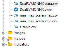
A csv file named DualSVMONNX-data.csv was created under the MQL5 directory Files.
Notice at the end of the function SendDataToONNX !!
I also saved the normalization parameters,
normalize_x.min_max_scaler.min.Swap(params);
matrix_utils.WriteCsv("min_max_scaler.min.csv",params,result,false,8);
normalize_x.min_max_scaler.max.Swap(params);
matrix_utils.WriteCsv("min_max_scaler.max.csv",params,result,false,8);
This is because the normalization parameters that were once used need to be used all over again to get the best predictions from the model, saving them would help us keep track of our data normalization parameter values, The CSV files will be in the same folder as the dataset and we'll also keep the ONNX model there.
DualSVMONNX class instance | Initializing a class:
class DualSVMONNX:
    def __init__(self, dataset, c=1.0, kernel='rbf'):

        data = pd.read_csv(dataset) # reading a csv file
        np.random.seed(42)

        self.X = data.drop(columns=['target']).astype(np.float32) # dropping the target column from independent variable
        self.y = data["target"].astype(int) # storing the target variable in its own vector

        self.X = self.X.to_numpy()
        self.y = self.y.to_numpy()

        # Split the data into training and testing sets
        self.X_train, self.X_test, self.y_train, self.y_test = train_test_split(self.X, self.y, test_size=0.2, random_state=42)

        self.onnx_model_name = "DualSVMONNX" #our final onnx model file name for saving purposes really

        # Create a dual SVM model with a kernel

        self.svm_model = SVC(kernel=kernel, C=c)
Training the Dual SVM model in python
    def fit(self):

        self.svm_model.fit(self.X_train, self.y_train) # fitting/training the model

        y_preds = self.svm_model.predict(self.X_train)

        print("accuracy = ",accuracy_score(self.y_train, y_preds))
Once the model is trained let us see what the accuracy looks like after this code snippet is run.
outputs:
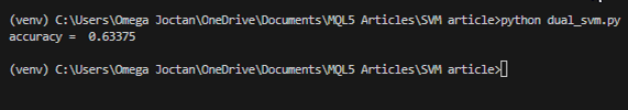
We got a 63% accuracy which tells us the SVM model for classifying this particular problem is average at best, however, I am suspicious let me run a cross-validation to prove if the accuracy is what it is supposed to be:
        scores = cross_val_score(self.svm_model, self.X_train, self.y_train, cv=5)
        mean_cv_accuracy = np.mean(scores)

        print(f"\nscores {scores} mean_cv_accuracy {mean_cv_accuracy}")
outputs:
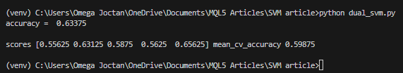
What does this cross-validation result mean?
There isn't a large variation between the outcome when the model is run with different parameters, this tells us our model is just on the right track the average accuracy we could get is 59.875 which isn't far away from 63.3 we got.
Converting SVC model from sklearn to ONNX and saving.
    def saveONNX(self):

        initial_type = [('float_input', FloatTensorType(shape=[None, 4]))]  # None means we don't know the rows but we know the columns for sure, Remember !! we have 4 independent variables
        onnx_model = convert_sklearn(self.svm_model, initial_types=initial_type) # Convert the scikit-learn model to ONNX format

        onnx.save_model(onnx_model, dataset_path + f"\\{self.onnx_model_name}.onnx") #saving the onnx model
outputs: NB: The model was saved under MQL5/Files directory
Below, is how the ONNX file looks when opened in MetaEditor. It is important that you pay attention to what I'm about to explain;

See the inputs section; You have the float_input which explains that this is an input of float types, next to it is tensor this tells us we might need to feed the OnnxRun function with a matrix or a vector as they are both tensors, at the end you see (?, 4) this is the input size a question mark stands for the number of rows is unknown while the number of columns is 4 This applies to the rest of the sections however you see the Outputs section.
It has two nodes one gives us the predicted labels -1 or 1 in this case they are of INT64 type or just INT in mql5.
The other node which gives us the probabilities, this is a tensor of float types it has unknown rows but 2 columns so an nx2 matrix can be used to extract the values here or just a vector sized >= 2
Since there are two nodes in the output we can extract the outputs twice:
   long outputs_0[] = {1};
   if (!OnnxSetOutputShape(onnx_handle, 0, outputs_0)) //giving the onnx handle first node output shape
     {
       Print(__FUNCTION__," Failed to set the output shape Err=",GetLastError());
       return false;
     }

   long outputs_1[] = {1,2};
   if (!OnnxSetOutputShape(onnx_handle, 1, outputs_1)) //giving the onnx handle second node output shape
     {
       Print(__FUNCTION__," Failed to set the output shape Err=",GetLastError());
       return false;
     }
On the other hand, we can extract a single input node we have.
   const long inputs[] = {1,4};

   if (!OnnxSetInputShape(onnx_handle, 0, inputs)) //Giving the Onnx handle the input shape
     {
       Print(__FUNCTION__," Failed to set the input shape Err=",GetLastError());
       return false;
     }
This ONNX code was extracted from the LoadONNX function given below:
bool CDualSVMONNX::LoadONNX(const uchar &onnx_buff[], ENUM_ONNX_FLAGS flags=ONNX_NO_CONVERSION)
 {
   onnx_handle =  OnnxCreateFromBuffer(onnx_buff, flags); //creating onnx handle buffer

   if (onnx_handle == INVALID_HANDLE)
    {
       Print(__FUNCTION__," OnnxCreateFromBuffer Error = ",GetLastError());
       return false;
    }

//---

   const long inputs[] = {1,4};

   if (!OnnxSetInputShape(onnx_handle, 0, inputs)) //Giving the Onnx handle the input shape
     {
       Print(__FUNCTION__," Failed to set the input shape Err=",GetLastError());
       return false;
     }

   long outputs_0[] = {1};
   if (!OnnxSetOutputShape(onnx_handle, 0, outputs_0)) //giving the onnx handle first node output shape
     {
       Print(__FUNCTION__," Failed to set the output shape Err=",GetLastError());
       return false;
     }

   long outputs_1[] = {1,2};
   if (!OnnxSetOutputShape(onnx_handle, 1, outputs_1)) //giving the onnx handle second node output shape
     {
       Print(__FUNCTION__," Failed to set the output shape Err=",GetLastError());
       return false;
     }

   return true;
 }
Take a closer look at the function you may notice we are missing on loading the normalization parameters which are crucial for standardizing the new input data so that it matches the dimensions of the trained data that the model is already familiar with.
We can Load the parameters from a CSV file, that will work smoothly during live trading however, this method might become complicated and not always work as effectively for the strategy tester, let us copy the normalization parameters to our EA code manually at least for now so that we end up with the normalization parameters inside our EA. First lets modify the LoadONNX function, so that it takes on the input vectors max and min which plays a huge part in Min Max Scaler.
bool CDualSVMONNX::LoadONNX(const uchar &onnx_buff[], ENUM_ONNX_FLAGS flags, vectorf &norm_max, vectorf &norm_min)
At the end of the function I introduced.
normalize_x = new CPreprocessing<vectorf,matrixf>(norm_max, norm_min); //Load min max scaler with parameters
Copying and Pasting the normalization Parameters from CSV files to EA's.
Let us train and try testing the model the same way we did using Python, the purpose of this is to make sure we are on the same path in both languages.
Inside OnInit function of svm test.mq5
vector min_v = {14.32424641,1.04674852,1.04799891,1.04392886};
vector max_v = {86.28263092,1.07385755,1.07907069,1.07267821};
//+------------------------------------------------------------------+
//| Expert initialization function                                   |
//+------------------------------------------------------------------+
int OnInit()
  {
//---
    rsi_handle = iRSI(Symbol(),PERIOD_CURRENT, rsi_period, PRICE_CLOSE);
    bb_handle = iBands(Symbol(), PERIOD_CURRENT, bb_period, 0 , bb_deviation, PRICE_CLOSE);


      vector y_train,
             y_test;

    // float values

      matrixf datasetf = GetTrainTestData<float>();
      matrixf x_trainf,
              x_testf;

      vectorf y_trainf,
              y_testf;

//---

      matrix_utils.TrainTestSplitMatrices(datasetf,x_trainf,y_trainf,x_testf,y_testf,0.8,42); //split the data into training and testing samples

      vectorf max_vf = {}, min_vf = {}; //convertin the parameters into float type
      max_vf.Assign(max_v);
      min_vf.Assign(min_v);

      dual_svm.LoadONNX(SVMModel, ONNX_DEFAULT, max_vf, min_vf);

      y_train.Assign(y_trainf);
      y_test.Assign(y_testf);

      vector train_preds = dual_svm.Predict(x_trainf);
      vector test_preds = dual_svm.Predict(x_testf);

      Print("\n<<<<< Train Classification Report >>>>\n");
      metrics.confusion_matrix(y_train, train_preds);

      Print("\n<<<<< Test  Classification Report >>>>\n");
      metrics.confusion_matrix(y_test, test_preds);


   return(INIT_SUCCEEDED);
  }
outputs:
RP      0       17:08:53.068    svm test (EURUSD,H1)    <<<<< Train Classification Report >>>>
HE      0       17:08:53.068    svm test (EURUSD,H1)
MR      0       17:08:53.068    svm test (EURUSD,H1)    Confusion Matrix
IG      0       17:08:53.068    svm test (EURUSD,H1)    [[245,148]
CO      0       17:08:53.068    svm test (EURUSD,H1)     [150,257]]
NK      0       17:08:53.068    svm test (EURUSD,H1)
DE      0       17:08:53.068    svm test (EURUSD,H1)    Classification Report
HO      0       17:08:53.068    svm test (EURUSD,H1)
FI      0       17:08:53.068    svm test (EURUSD,H1)    _    Precision  Recall  Specificity  F1 score  Support
ON      0       17:08:53.068    svm test (EURUSD,H1)    1.0    0.62     0.62     0.63       0.62     393.0
DP      0       17:08:53.068    svm test (EURUSD,H1)    -1.0    0.63     0.63     0.62       0.63     407.0
JG      0       17:08:53.068    svm test (EURUSD,H1)
FR      0       17:08:53.068    svm test (EURUSD,H1)    Accuracy                                   0.63
CK      0       17:08:53.068    svm test (EURUSD,H1)    Average   0.63    0.63    0.63      0.63    800.0
KI      0       17:08:53.068    svm test (EURUSD,H1)    W Avg     0.63    0.63    0.63      0.63    800.0
PP      0       17:08:53.068    svm test (EURUSD,H1)
DH      0       17:08:53.068    svm test (EURUSD,H1)    <<<<< Test  Classification Report >>>>
PQ      0       17:08:53.068    svm test (EURUSD,H1)
EQ      0       17:08:53.068    svm test (EURUSD,H1)    Confusion Matrix
HJ      0       17:08:53.068    svm test (EURUSD,H1)    [[61,31]
MR      0       17:08:53.068    svm test (EURUSD,H1)     [40,68]]
NH      0       17:08:53.068    svm test (EURUSD,H1)
DP      0       17:08:53.068    svm test (EURUSD,H1)    Classification Report
HL      0       17:08:53.068    svm test (EURUSD,H1)
FF      0       17:08:53.068    svm test (EURUSD,H1)    _    Precision  Recall  Specificity  F1 score  Support
GJ      0       17:08:53.068    svm test (EURUSD,H1)    -1.0    0.60     0.66     0.63       0.63     92.0
PO      0       17:08:53.068    svm test (EURUSD,H1)    1.0    0.69     0.63     0.66       0.66     108.0
DD      0       17:08:53.068    svm test (EURUSD,H1)
JO      0       17:08:53.068    svm test (EURUSD,H1)    Accuracy                                   0.65
LH      0       17:08:53.068    svm test (EURUSD,H1)    Average   0.65    0.65    0.65      0.64    200.0
CJ      0       17:08:53.068    svm test (EURUSD,H1)    W Avg     0.65    0.65    0.65      0.65    200.0
We got 63% the same accuracy value we got from our Python script. Isn't that wonderful !!!
This is what the predict function looks like on the inside:
int CDualSVMONNX::Predict(vectorf &inputs)
 {
    vectorf outputs(1); //label outputs
    vectorf x_output(2); //probabilities

    vectorf temp_inputs = inputs;

    normalize_x.Normalization(temp_inputs); //Normalize the input features

    if (!OnnxRun(onnx_handle, ONNX_DEFAULT, temp_inputs, outputs, x_output))
      {
         Print("Failed to get predictions from onnx Err=",GetLastError());
         return (int)outputs[0];
      }

   return (int)outputs[0];
 }
It runs the ONNX file to get the predictions and returns an integer for the predicted label.
Finally, I had to implement a simple strategy to allow us to test both of the Support Vector Machine models in the strategy tester. The strategy is simple if the predicted class by SVM == 1 open buy trade otherwise if the predicted class == -1 open a sell trade.
Results in the strategy tester:
for Linear Support Vector Machine:
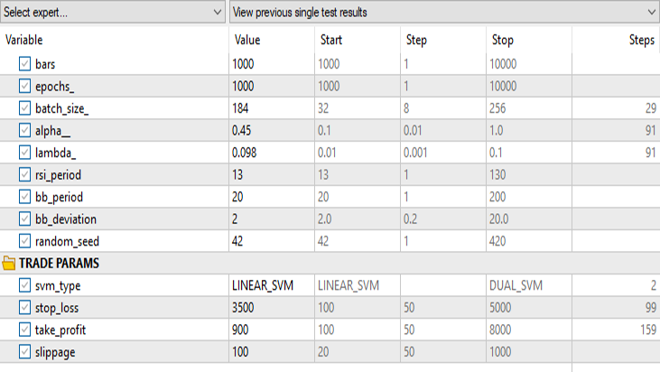
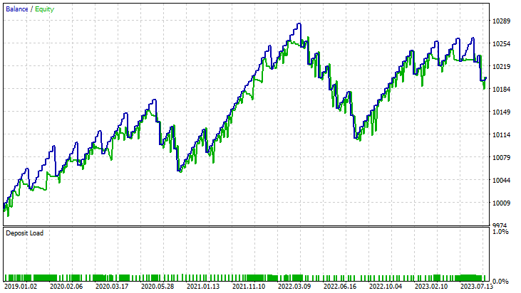
for Dual Support Vector Machine:
Keeping all the inputs the same except the svm_type.
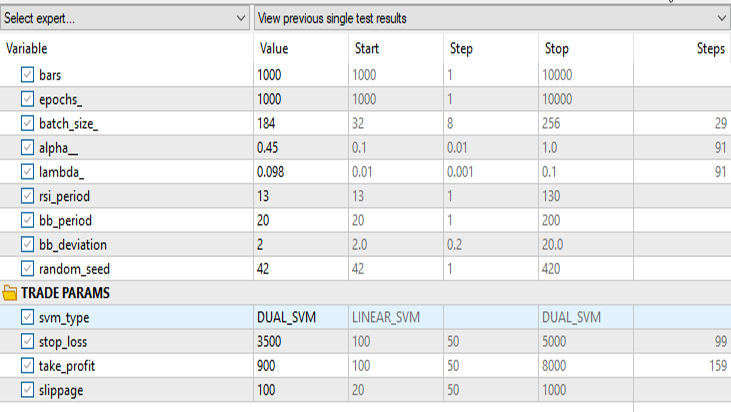
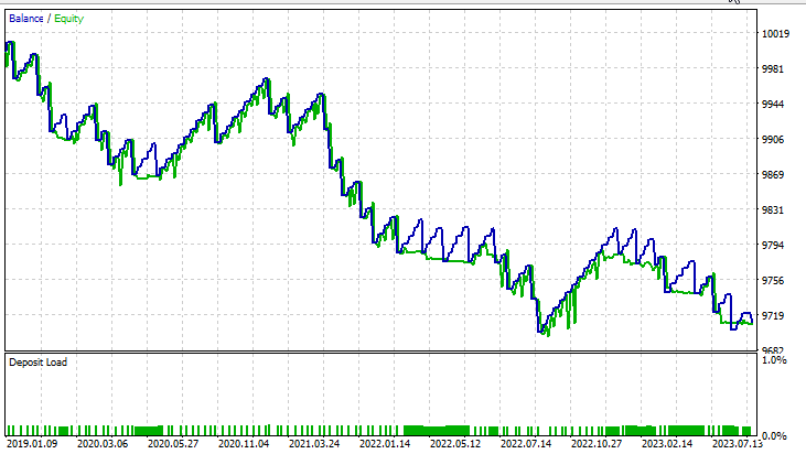
The dual SVM did not perform well with the inputs that worked for Linear SVM, there might be a need to optimize further and explore why the ONNX model did not converge but, that's a topic for another article.
Final Thoughts
Advantages of SVM Models:
- Effective in High-Dimensional Spaces: SVMs perform well in high-dimensional spaces, making them suitable for financial datasets with numerous features, such as trading indicators and market variables.
- Robust to Overfitting: SVMs are less prone to overfitting, providing a more generalized solution that can better adapt to unseen market conditions.
- Versatility in Kernels: SVMs offer versatility through different kernel functions, allowing traders to experiment with various strategies and adapt the model to specific market patterns.
- Strong Performance in Nonlinear Scenarios: SVMs excel in capturing nonlinear relationships within data, a crucial aspect when dealing with complex financial markets.
Disadvantages:
- Sensitivity to Noise: SVMs can be sensitive to noisy data, impacting their performance and making them more susceptible to erratic market behavior.
- Computational Complexity: Training SVM models can be computationally expensive, especially with large datasets, limiting their scalability in certain real-time trading scenarios.
- Need for Quality Feature Engineering: SVMs heavily rely on feature engineering, requiring domain expertise to select relevant indicators and preprocess data effectively.
- Average Performance: As we have seen, SVM models achieved average accuracy results of 63% for dual SVM and 59% for linear SVM. While these models may not outperform some advanced machine-learning techniques, they still offer a reasonable starting point for MQL5 traders.
The Decline in Popularity:
Despite their historical success, SVMs have experienced a decline in popularity in recent years. This is attributed to:
- Emergence of Deep Learning: The rise of deep learning techniques, particularly neural networks, has overshadowed traditional machine learning algorithms like SVMs due to their ability to automatically extract hierarchical features.
- Increased Availability of Data: With the increasing availability of vast financial datasets, deep learning models, which thrive on large amounts of data, have become more appealing.
- Computational Advances: The availability of powerful hardware and distributed computing resources has made it more feasible to train and deploy complex deep-learning models.
In conclusion, while SVM models may not be the cutting-edge solution, their use in MQL5 trading environments is justified. Their simplicity, robustness, and adaptability make them a valuable tool, especially for traders with limited data or computational resources. It's essential for traders to consider SVMs as part of a broader toolkit, potentially complementing them with newer machine-learning approaches as market dynamics evolve.
Best Regards, Peace out.
| File | Description | Usage |
|---|---|
| dual_svm.py | python script | It has Dual SVM implementation in python |
| GetDataforONNX.mq5 | mql5 script | Can be used to collect, normalize and store the data in a csv file located under MQL5/Files |
| preprocessing.mqh | mql5 include file | Contains class and functions for normalizing and standardizing the input data |
| matrix_utils.mqh | mql5 include file | A library with additional matrix operations |
| metrics.mqh | mql5 include file | A library containing additional functions to analyze ML models performance |
| svm test.mq5 | EA | An expert Advisor for testing all the code we have in the article |
The code used in this article can also by found on my GitHub repo.
Warning: All rights to these materials are reserved by MetaQuotes Ltd. Copying or reprinting of these materials in whole or in part is prohibited.
This article was written by a user of the site and reflects their personal views. MetaQuotes Ltd is not responsible for the accuracy of the information presented, nor for any consequences resulting from the use of the solutions, strategies or recommendations described.

- Free trading apps
- Over 8,000 signals for copying
- Economic news for exploring financial markets
You agree to website policy and terms of use