The price movement model and its main provisions (Part 2): Probabilistic price field evolution equation and the occurrence of the observed random walk

Introduction

After introducing the basics of the wave probabilistic price model, I was going to immediately proceed to the price random walk in the wave probabilistic field while coming up with conclusions that are practically important for trading. But in the forum discussion of the first part of the article, users asked me some important questions boiling down to the following: "How do price random walks correlate with the wave model of its evolution and how are the corresponding instantaneous states (chart values) of the price interpreted from the standpoint of this model?" So I decided to answer these questions in a separate article, while presenting all the accompanying theoretical concepts, which are also extremely important, since they are used to predict the wave probabilistic field.

Probabilistic price field evolution equation

Before establishing the essence of the relationship between price random walks and its probabilistic wave movement, let me first present in more detail the analytics of the latter with the equation the wave field adheres to. 

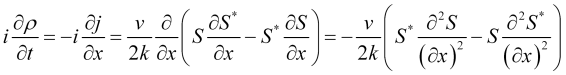
Price probabilistic field  equation

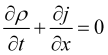           ,                                                                                                    (1)

where ,    is a price field probability stream, while - stream velocity. Considering the equation

                                                                                                                         (2)

for the operator proper values for the wave vector and their real character, the probability stream can be set as

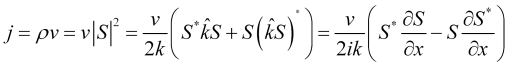             ,    (3)

where  is a wave vector of the price field.

     

The  wave field defines the true state of the price. Let's assume that the wave field function is smooth stipulating the existence of its derivative by time. In this case, the future value of the wave field function can be found via its derivative. If the market is not affected by strong external influences that violate the smoothness, the knowledge of the  wave field at the current moment of time allows it to be calculated at subsequent moments of time, which is true within a time interval limited by strong external influences on the market. In this case, the price evolution equation looks as follows

           ,                                                                                                         (4) 

where  is a linear (due to the principle of superposition of the wave field partial components) evolution operator.

 

 integral of the price probability density over the entire price scale is a constant or unity if the probability density is normalized, therefore:

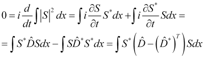                                           (5)

where  is a transposition operation. Therefore,  

         ,                                                                                               (6)

in other words, the Hermitian evolution operator. Let's find its form.

 

Using (4) and (6), we get

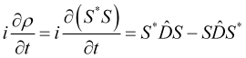                                                                          (7)

On the other hand, from (1) and (3), we have

         (8)

When comparing (7) and (8), we can see that the evolution operator looks as follows

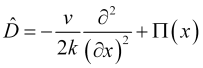              ,                                                                          (9)

where means the potential, in which the probabilistic price field is distributed. In this case, the price wave field evolution equation looks as follows

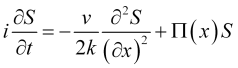              ,                                                                (10)

which is identical to the one-dimensional Schrödinger equation in its analytical content. Indeed, given that in quantum mechanics the momentum , the factor in the (10) equation for the quantum theory is equal to 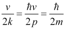.  By replacing the factor in (10) with its quantum mechanical counterpart and multiplying (10) by the Plank constant, as well as replacing   with  more usual for physicists, we get

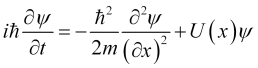                                                                         (10.1)

the one-dimensional Schrödinger equation, where the quantum mechanical potential is related to the price field potential by the relation since the  potential has the dimension of frequency, and the quantum mechanical potential has the dimension of energy.   

Apparently, equation (10) is a general equation for the evolution of probabilistic wave fields that can be of different origin.

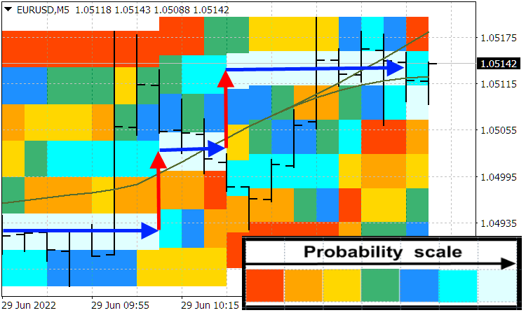
If the  potential looks like a deep hole the price wave is unable to overcome reflecting from the hole walls (and slightly penetrating into the hole due to exponential attenuation), in other words, if the price movement is finite, then, in accordance with the elementary quantum mechanical solutions of this problem, we get a discrete range of prices.  This will also explain (even in this simplest linear model) the existence of price levels, between which the price moves in jumps, or spikes. Knowing the current potential, we can easily find these price levels, between which the price moves in jumps. Practice shows that such price levels do exist. The following screenshot shows these price levels (blue arrows) and price spikes (red arrows). We can also see that during price spikes, the price value becomes more uncertain compared to its value at the price level.

Probabilities distribution of price indicator

Upcoming price spike criterion

In the first part of the article, I stated that price spikes can be caused both by external and internal causes. While in the former case it is impossible to predict such spikes based on the quote history, in the latter case (which is by no means less common), there is a chance to detect them. Let us dwell on the analytics of identifying the second-order spike approximation. For the convenience of further analysis, the (N) equation of the first part will be shown as (I.N).  Let us first prove that the (I.16) uncertainty relation minimizes the Morlet wavelet, the proof of which was omitted in the first part for brevity sake. 

The (I.16) relation reaches the minimum at , which is a root of (I.15) in case of the zero discriminant.  Enter   and operators, then (I.11) for its minimum value can be written as

              .                                                                  (11)

 

From (11), it is implied that

                                                                                                           (12)

or

              ,                                                                                     (13)

which has the solution 

                 ,                                                                               (14)

The (14) relation considering that the wave number operator fits the proper value equation

                 ,                                                                                                   (15)

which has the solution and yields the (I.17) equation after normalization or   

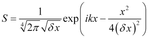                  .                                                  (16)               

 

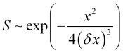
The (I.16) minimum or the  minimum product of uncertainties is reached when the  state vector does not change during the Fourier transform, which takes place if the probability field has the form (16). Gauss, which models the harmonic component of the field in both representations (coordinate and frequency ones), is symmetrical. The density of the price probability distribution around its average in the horizontal segment of the price movement or before a spike is also more or less symmetrical. However, during the spike, the probability density function, and hence, the envelope of the  price probability field becomes asymmetric, which indicates an increase in the product . Thus, an increase in  can serve as a criterion for a possible price spike, if it is caused by internal market processes.

 

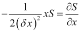
Then in accordance with the (11) relation, which minimizes , we can conclude that the increase of the fundamentally positive function 

                                                                                                        (17)

can serve as an upcoming price spike criterion.

Reducible price values and their random walks

The problem of the essence of the relationship between the price visible on the chart and its wave probabilistic field is very complex and requires not only the consideration of purely technical aspects of price formation but also a deep philosophical analysis.  

First, let's talk about the purely technical aspects of pricing. Quote charts display only the price values that (1) are either provided by a liquidity provider or aggregator to a broker or a dealer, (2) or formed by a bank or a prime broker. Let's call these visible price values reducible. The emergence of such reduced prices has its own history, which is important for understanding the complexity of the relationships of their formation. The prices are formed by supply and demand, which were first formed by large banks under the supervision of a national regulator.

These banks were supposed to be guided by global supply and demand. Thomson Reuters took over the collection and processing of information on Forex rates. The company supplied this information in real time based on major transactions of many international financial organizations, thus setting a benchmark of purchase and sale prices for banks. With the advent of the Internet, Forex brokers began to remotely open accounts for their clients and arrange trading on cloud platforms. Currently, banks and large brokers (called prime brokers since they deal with large volumes) have begun to independently form exchange rates for their clients refusing the services of liquidity providers. But Thomson Reuters (and then a number of other companies) offered its services to small clients by combining orders on one online platform with the formation of an integral order book, where impersonal orders are summed up by price levels, which is the essence of the currency liquidity aggregator. 

There are currently two main types of access to foreign exchange liquidity.

1. Market making – a foreign exchange liquidity provider, which fulfills orders of brokers' clients who have agreements with that provider. These banks work only with large brokers and volumes,
2. Liquidity aggregators are used by small brokers.

The main liquidity providers have complete information about their depth of market with bid and ask prices and their volumes. Based on the lower boundary of sell offers, the provider determines the Ask price for its customers, and from the upper boundary of buy offers, the provider forms the Bid price. In other words, the reducible price, in fact, consists of two components. Speaking about the wave field of the price, we mean one of these components. 

The corresponding prices, in essence, are determined by all those traders, associated with the quotes provider, who form their orders based on their market data. All market participants receive their data from a single information space for the whole world. Data is obtained almost instantaneously. Therefore, the price is reduced not only by the provider alone but also by its multiple clients whose role in the formation of price values is much greater than the role of the provider itself. Besides, due to the unity of the information space and the instant access of clients to it, the prices reduced by different liquidity providers turn out to be much similar.

Now let's talk about the ontology of the relation between reducible prices and emergent price waves. To reveal the topic, let's make a block diagram presenting the main elements of the complex system of relationships between the probabilistic and the reducible elements for the market.

 

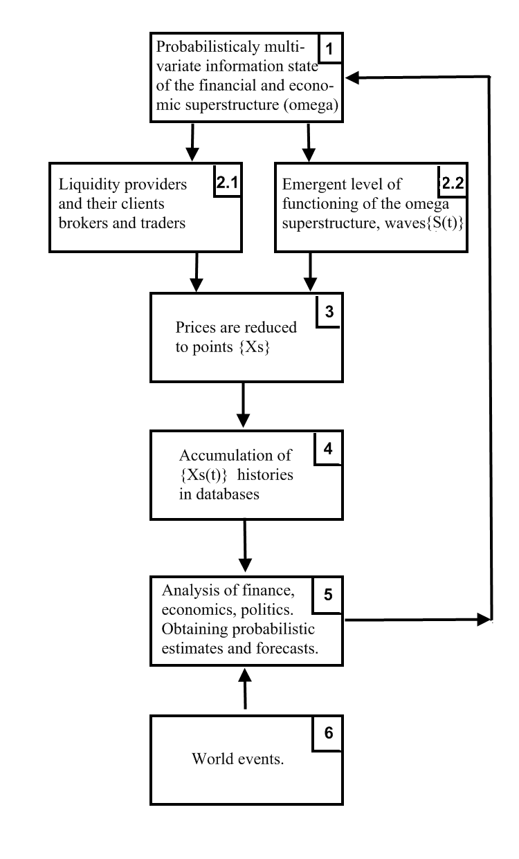
 price probability waves propagating in their emergent space are, in fact, generated by the entire financial and economic superstructure of the human civilization, which can be symbolically set as  , which corresponds to the {1 → 2.2} connection on the block diagram. The state of the financial and economic superstructure {1} (the diagram blocks are indicated by curly brackets in the text) is probabilistically multivariate due to the {5 → 1} feedback, where block {5} (more precisely, financial, economic and political analysts from all over the world) generates probabilistic forecasts and estimates. Due to the probabilistic state of the superstructure {1} (this is all we know about it), the emergent world {2.2} of price waves generated by it is also probabilistic, which exhaustively reflects the state of this superstructure.  The clients of a  liquidity provider also get financial data they are interested in from the superstructure {1} (more precisely, from experts describing its state). However, they choose private and unambiguous information close to their understanding of the market from the multivariate data of the superstructure {1}, whose selection can be interpreted as random (since an external expert assessing the situation is not aware of the mindset of all those clients). The {1 → 2.1} connection clearly does not reflect the superstructure {1} exhaustively and instead randomly selects one of its sides. The liquidity provider reduces the price of the symbol based on the market depth formed for it by its clients' orders, which corresponds to the {2.1 → 3} relation of the block diagram. However, if we look at the reality through the lens of the emergent probabilistic fields summarizing all particularities {2.2} (with no regard to the actions and motivations of individual traders), it turns out that the same  price is reduced from the wave field randomly.

Thus, considering reality in different ways (here the role of the observer manifests itself in reducing the very algorithm for the formation of the observed reality), it is possible to identify two facets of the same, inherently random, reduction phenomenon, when randomness at the {1 → 2.1 → 3} facet occurs at stage {1 → 2.1}, while at the {1 → 2.2 → 3} facet, it occurs during {2.2 → 3}. However, price evolution can be predicted only by using the representation of the emergent space, which exhaustively reflects the superstructure {1}, since the price reducing by the liquidity provider is based only on a random reflection of one of the particular parties, at the same time losing the main array of the data necessary for the forecast. I want to emphasize that only a wave field is able to express the price exhaustively. In other words, the  relation is not only more general than {1 → 2.1}, but is also more informative. Therefore, price reduction is an incomplete or simplified (reduction is from Latin 'reductio', which has a meaning of 'simplification' among others) reflection of its price field.

By means of the {3 → 4 → 5 → 1 → 2.2} connection chain, reduced prices have the opposite effect on  and the S(t) wave field. But market reduction, unlike state reduction in quantum mechanics, does not lead to the collapse of the wave function. Instead, it can only slightly affect the subsequent price evolution described by the equation (10). In my opinion, the energy of the device used during an experiment with a micro object is incomparably greater than the energy of the micro object itself leading to a strong compression of the micro object state (or its localization in a specific spatial point or state).

If we are talking about financial or price reduction, then the traders' lots the liquidity provider relies on when reducing the price of a certain instrument, is incomparably less than the total volume of this instrument in the entire financial market. Thus, the effect on the wave field of such an instrument during its reduction is small. Summarizing the above, we can conclude that the evolution of the price wave field and its quote history are two forms (full implicit and abbreviated explicit) of existence of the same price phenomenon. Starting from the representation of an independent emergent functioning of the market, we can say that the ensemble of quote histories of a certain instrument, reduced by all providers of its liquidity, is an incomplete reflection of the evolution of the price wave field of the same instrument in the same history section.

Finally, we can already reveal the essence of the price random walk from the perspective of its wave field. Let's assume that the current price probability density sets the  probability of its reduction on a small interval . Different liquidity providers may offer slightly different prices for the same instrument. But it is obvious that the price close to the average value is reduced most often.

                                                                                   (18)

(not to be confused with , which does not lag behind, with a moving average that lags by half of its averaging period). With each such reduction (as well as with the act of quantum mechanical measurement, which is its analogue), the observed price fluctuates around the average value (18) with the squared uncertainty already established in the first part

            .                                                                                   (19)

which, in fact, gives rise to the process of price random walk already visible on the monitors. Some random spikes caused by reduction and even their small sequences (which may even form sections similar to trends, see True and illusory currency market trends, which are sections of a false trend making them unsuitable for making a stable profit), are, generally, not very informative (in the sense of little use for trading). What is really important is a movement of the  average and their distribution around it. In the process of the average movement and reduction, the sequences are formed, where  are random values that (with the probability corresponding to the distribution) fall into the type intervals, which is the expression of the price random walk. The average, near which the reduced price randomly “jumps”, is formed by the wave probabilistic field, so the process of generating the  sequence can be conditionally called the price random walk in the wave probability field.

I want to stress that the average and the probability distribution are formed by no means by standard statistical processes, but by waves of probability amplitudes interfering with each other in emergent space. Strictly speaking, the methods of ordinary standard statistics are poorly applicable to the market and yield large errors there. But considering that we are unable to see the price wave field yet, the practically defined (from price charts) probabilities of directions of these random spikes allow us to roughly judge the evolution of the average. This, in turn, allows us to develop an approach to identifying the optimal market trading parameters (within the simplified model). We will consider that in the next article.

Conclusion

What we see every day on quote charts is a fairly detailed reflection of the real quantum world, which can be described with quantum laws (wave fields, specific reduction processes, the Schrödinger equation, etc.) and quantum logic! This quantum world is created by a huge group of market participants and exists in an emergent way as a qualitatively different superstructure over the activities of this group. The knowledge of this fact and the corresponding mathematical apparatus will allow us to create much more efficient products - quantum EAs and indicators based on the equation of the evolution of the corresponding wave fields.