Статистический арбитраж с прогнозами

MetaTrader 5 — Торговые системы | 19 сентября 2024, 14:21

2 215

Javier Santiago Gaston De Iriarte Cabrera

Введение

Статистический арбитраж — это сложная финансовая стратегия, которая использует математические модели для извлечения выгоды из неэффективности цен между взаимосвязанными финансовыми инструментами. Этот подход, обычно применяемый к акциям, облигациям или производным финансовым инструментам, требует глубокого понимания корреляции, коинтеграции и коэффициента Пирсона — важнейших инструментов для выявления и использования рыночных возможностей.

Корреляция в финансах измеряет, насколько тесно две ценные бумаги движутся по отношению друг к другу, количественно определяя степень их взаимосвязи. Положительная корреляция указывает на то, что ценные бумаги обычно движутся в одном направлении, тогда как отрицательная означает, что они движутся в противоположных направлениях. Трейдеры анализируют эти взаимосвязи, чтобы прогнозировать будущие движения цен.

Коинтеграция, более тонкое статистическое свойство, выходит за рамки корреляции, исследуя, остается ли линейная комбинация двух или более переменных временного ряда стабильной с течением времени. Проще говоря, хотя отдельные ценные бумаги могут следовать разным путям, их относительные движения связаны неким равновесием, к которому они имеют тенденцию возвращаться. Эта концепция имеет решающее значение в парной торговле, цель которой — определить пары акций, цены которых исторически движутся вместе и, как ожидается, будут продолжать двигаться в том же направлении.

Коэффициент Пирсона - статистическая мера, которая вычисляет силу и направление линейной связи между двумя переменными. Значения коэффициента Пирсона находятся в диапазоне от -1 до 1, где 1 означает идеальную положительную линейную связь, -1 — идеальную отрицательную линейную связь, а 0 — отсутствие линейной связи. В статистическом арбитраже высокое абсолютное значение коэффициента Пирсона между двумя активами может указывать на потенциальную возможность торговли, если они вернутся к долгосрочному среднему соотношению.

Трейдеры, реализующие стратегии статистического арбитража, используют алгоритмы и высокочастотные торговые системы для мониторинга и исполнения сделок. Эти системы способны обрабатывать огромные объемы данных для быстрого обнаружения аномалий в отношениях цен на активы. Стратегия предполагает, что цены коррелируемых активов сойдутся к своему историческому среднему значению, что позволит трейдеру получить прибыль от корректировки цен.

Однако успех статистического арбитража зависит не только от сложных математических моделей, но и от способности трейдера интерпретировать данные и корректировать стратегии в зависимости от меняющихся рыночных условий. Такие факторы, как внезапные экономические изменения, рыночные настроения или политические события, могут нарушить даже самые стабильные отношения, повышая уровень риска.

Объяснение с простыми примерами

Корреляция измеряет, как связаны два объекта. Представьте, что вы вместе с вашим лучшим другом всегда ходите в кино по субботам. Это пример корреляции: когда вы идете в кино, ваш друг тоже идет. Если корреляция положительная, это означает, что при увеличении одного показателя увеличивается и другой. Если отрицательная, один увеличивается, а другой уменьшается. Если корреляция равна нулю, это означает, что между объектами нет никакой связи.

Коинтеграция - статистическая концепция, используемая для описания ситуации, когда две или более переменных имеют некоторую долгосрочную взаимосвязь, даже если они могут колебаться независимо в краткосрочной перспективе. Представьте себе двух пловцов, связанных веревкой: они могут свободно плавать в бассейне, но не могут отдаляться далеко друг от друга. Коинтеграция указывает на то, что, несмотря на временные различия, эти переменные всегда будут возвращаться к общему долгосрочному равновесию или тренду.

Коэффициент Пирсона измеряет, насколько линейно связаны две переменные. Если коэффициент близок к +1, это указывает на прямую зависимость: при увеличении одной переменной увеличивается и другая. Коэффициент, близкий к -1, означает, что при увеличении одной переменной другая уменьшается, что указывает на обратную зависимость. Значение 0 означает отсутствие линейной связи. Например, измерение температуры и объема продаж прохладительных напитков может помочь понять, как связаны эти факторы, с помощью коэффициента Пирсона.

Подводя итог, можно сказать, что статистический арбитраж — это сложная, но потенциально прибыльная торговая стратегия, сочетающая в себе элементы экономики, финансов и математики. Она требует не только понимания статистических терминов, но и способности применять высокоскоростные алгоритмы для анализа рынка и исполнения сделок.

Расчет

Чтобы узнать, какие пары коинтегрированы и коррелированы, вы можете использовать следующий python-код.

import MetaTrader5 as mt5
import pandas as pd
from scipy.stats import pearsonr
from statsmodels.tsa.stattools import coint
import numpy as np

# Connect with MetaTrader 5
if not mt5.initialize():
    print("Failed to initialize MT5")
    mt5.shutdown()

# Get the list of symbols
symbols = mt5.symbols_get()
symbols = [s.name for s in symbols if s.name.startswith('EUR') or s.name.startswith('USD') or s.name.endswith('USD')]  # Filtrar símbolos por ejemplo

# Download historical data and save in dictionary
data = {}
for symbol in symbols:
    rates = mt5.copy_rates_from_pos(symbol, mt5.TIMEFRAME_D1, 0, 365)  # Último año, diario
    if rates is not None:
        df = pd.DataFrame(rates)
        df['time'] = pd.to_datetime(df['time'], unit='s')
        data[symbol] = df.set_index('time')['close']

# Close connection with MT5
mt5.shutdown()

# Calculate the Pearson coefficient and test for cointegration for each pair of symbols
cointegrated_pairs = []
for i in range(len(symbols)):
    for j in range(i + 1, len(symbols)):
        if symbols[i] in data and symbols[j] in data:
            common_index = data[symbols[i]].index.intersection(data[symbols[j]].index)
            if len(common_index) > 30:  # Asegurarse de que hay suficientes puntos de datos
                corr, _ = pearsonr(data[symbols[i]][common_index], data[symbols[j]][common_index])
                if abs(corr) > 0.8:  # Correlación fuerte
                    score, p_value, _ = coint(data[symbols[i]][common_index], data[symbols[j]][common_index])
                    if p_value < 0.05:  # P-valor menor que 0.05
                        cointegrated_pairs.append((symbols[i], symbols[j], corr, p_value))

# Filter and show only cointegrated pairs with p-value less than 0.05
print(f'Total pairs with strong correlation and cointegration: {len(cointegrated_pairs)}')
for sym1, sym2, corr, p_val in cointegrated_pairs:
    print(f'{sym1} - {sym2}: Correlación={corr:.4f}, P-valor de Cointegración={p_val:.4f}')

Результаты:

Total pairs with strong correlation and coitegration: 54
EURUSD - USDBGN: Correlación=-0.9957, P-valor de Cointegración=0.0000
EURUSD - USDHRK: Correlación=-0.9972, P-valor de Cointegración=0.0000
GBPUSD - USDPLN: Correlación=-0.8633, P-valor de Cointegración=0.0406
GBPUSD - GBXUSD: Correlación=0.9998, P-valor de Cointegración=0.0000
GBPUSD - EURSGD: Correlación=0.8061, P-valor de Cointegración=0.0191
USDCHF - EURCHF: Correlación=0.8324, P-valor de Cointegración=0.0356
USDJPY - EURDKK: Correlación=0.8338, P-valor de Cointegración=0.0200
USDJPY - USDTHB: Correlación=0.9012, P-valor de Cointegración=0.0330
AUDUSD - USDCNH: Correlación=-0.8074, P-valor de Cointegración=0.0390
EURCHF - USDKES: Correlación=-0.9104, P-valor de Cointegración=0.0048
EURJPY - EURRON: Correlación=0.8177, P-valor de Cointegración=0.0333
EURJPY - USDCOP: Correlación=-0.9361, P-valor de Cointegración=0.0125
EURJPY - USDLAK: Correlación=0.9508, P-valor de Cointegración=0.0410
EURJPY - EURDKK: Correlación=0.8525, P-valor de Cointegración=0.0136
EURJPY - EURMXN: Correlación=-0.8785, P-valor de Cointegración=0.0172
EURJPY - USDTRY: Correlación=0.9564, P-valor de Cointegración=0.0102
EURNZD - NZDUSD: Correlación=-0.8505, P-valor de Cointegración=0.0455
EURNZD - EURDKK: Correlación=0.8242, P-valor de Cointegración=0.0017
EURCZK - USDCLP: Correlación=0.9655, P-valor de Cointegración=0.0001
USDCLP - USDCZK: Correlación=0.8972, P-valor de Cointegración=0.0147
USDCLP - USDARS: Correlación=0.8077, P-valor de Cointegración=0.0231
USDCLP - USDIDR: Correlación=0.8569, P-valor de Cointegración=0.0423
USDCLP - USDNGN: Correlación=0.8468, P-valor de Cointegración=0.0436
USDCLP - USDVND: Correlación=0.9021, P-valor de Cointegración=0.0194
USDCZK - USDIDR: Correlación=0.9005, P-valor de Cointegración=0.0086
USDCZK - USDVND: Correlación=0.8306, P-valor de Cointegración=0.0195
USDMXN - USDCOP: Correlación=0.8686, P-valor de Cointegración=0.0286
USDMXN - EURMXN: Correlación=0.9522, P-valor de Cointegración=0.0328
NZDUSD - USDSGD: Correlación=-0.8145, P-valor de Cointegración=0.0097
NZDUSD - USDTHB: Correlación=-0.8094, P-valor de Cointegración=0.0255
ADAUSD - KSMUSD: Correlación=0.9429, P-valor de Cointegración=0.0071
ALGUSD - LNKUSD: Correlación=0.8038, P-valor de Cointegración=0.0454
ATMUSD - MTCUSD: Correlación=0.9423, P-valor de Cointegración=0.0146
BTCUSD - SOLUSD: Correlación=0.9736, P-valor de Cointegración=0.0112
DGEUSD - GLDUSD: Correlación=0.8933, P-valor de Cointegración=0.0136
DGEUSD - USDGHS: Correlación=0.8562, P-valor de Cointegración=0.0101
EOSUSD - UNIUSD: Correlación=0.8176, P-valor de Cointegración=0.0051
ETCUSD - ETHUSD: Correlación=0.9745, P-valor de Cointegración=0.0009
ETCUSD - SOLUSD: Correlación=0.9206, P-valor de Cointegración=0.0093
ETCUSD - UNIUSD: Correlación=0.9236, P-valor de Cointegración=0.0249
ETHUSD - SOLUSD: Correlación=0.9430, P-valor de Cointegración=0.0074
UNIUSD - USDNGN: Correlación=0.8074, P-valor de Cointegración=0.0195
EURNOK - USDNOK: Correlación=0.9065, P-valor de Cointegración=0.0430
EURRON - USDCOP: Correlación=-0.8010, P-valor de Cointegración=0.0097
EURRON - USDCRC: Correlación=-0.8015, P-valor de Cointegración=0.0159
EURRON - USDLAK: Correlación=0.8364, P-valor de Cointegración=0.0349
GBXUSD - EURSGD: Correlación=0.8067, P-valor de Cointegración=0.0180
USDARS - USDVND: Correlación=0.8093, P-valor de Cointegración=0.0268
USDBGN - USDHRK: Correlación=0.9944, P-valor de Cointegración=0.0000
USDCOP - USDTRY: Correlación=-0.9548, P-valor de Cointegración=0.0160
USDCRC - EURDKK: Correlación=-0.8519, P-valor de Cointegración=0.0153
USDHRK - USDDKK: Correlación=0.9954, P-valor de Cointegración=0.0000
USDIDR - USDVND: Correlación=0.8196, P-valor de Cointegración=0.0417
USDSEK - USDSGD: Correlación=0.8346, P-valor de Cointegración=0.0264

Пары отсортированы.

Для проверки значений с помощью MetaTrader 5 у нас есть индикатор (Pearson.mq5):

//+------------------------------------------------------------------+
//|                                             PearsonIndicator.mq5 |
//|                    Copyright Javier S. Gastón de Iriarte Cabrera |
//|                                       https://www.mql5.com/en/users/jsgaston/news |
//+------------------------------------------------------------------+
#property copyright "Javier S. Gastón de Iriarte Cabrera"
#property link      "https://www.mql5.com/en/users/jsgaston/news/"
#property version   "1.00"
#property indicator_separate_window
#property indicator_buffers 1
#property indicator_color1 Red

input string Symbol2 = "GBPUSD";       // Second financial instrument
input int BarsBack = 100;              // Number of bars to include in correlation calculation

double CorrelationBuffer[];

//+------------------------------------------------------------------+
//| Custom indicator initialization function                         |
//+------------------------------------------------------------------+
int OnInit()
  {
   SetIndexBuffer(0, CorrelationBuffer, INDICATOR_DATA);
   PlotIndexSetInteger(0, PLOT_DRAW_TYPE, DRAW_LINE);
   PlotIndexSetString(0, PLOT_LABEL, "Pearson Correlation");
   IndicatorSetString(INDICATOR_SHORTNAME, "Pearson Correlation (" + Symbol() + " & " + Symbol2 + ")");
   return INIT_SUCCEEDED;
  }

//+------------------------------------------------------------------+
//| Custom indicator iteration function                              |
//+------------------------------------------------------------------+
int OnCalculate(const int rates_total,
                const int prev_calculated,
                const datetime &time[],
                const double &open[],
                const double &high[],
                const double &low[],
                const double &close[],
                const long &tick_volume[],
                const long &volume[],
                const int &spread[])
  {
   if (rates_total < BarsBack) return 0; // Ensure enough bars are present

   double prices1[], prices2[];
   ArrayResize(prices1, BarsBack);
   ArrayResize(prices2, BarsBack);

   // Copy historical data for primary symbol
   if (CopyClose(Symbol(), PERIOD_CURRENT, 0, BarsBack, prices1) <= 0)
      {
       Print("Error copying prices for ", Symbol());
       return 0;
      }
   // Copy historical data for secondary symbol
   if (CopyClose(Symbol2, PERIOD_CURRENT, 0, BarsBack, prices2) <= 0)
      {
       Print("Error copying prices for ", Symbol2);
       return 0;
      }

   // Calculate Pearson correlation for the entire buffer
   double correlation = CalculatePearsonCorrelation(prices1, prices2);
   Print("Pearson correlation: ", correlation);

   // Fill the buffer for the indicator
   for (int i = BarsBack; i < rates_total; i++)
     {
      CorrelationBuffer[i] = correlation;  // Update the buffer correctly
     }

   return(rates_total);
  }

//+------------------------------------------------------------------+
//| Calculate Pearson correlation coefficient                        |
//+------------------------------------------------------------------+
double CalculatePearsonCorrelation(double &prices1[], double &prices2[])
  {
   int length = BarsBack;
   double mean1 = 0, mean2 = 0;
   double sum1 = 0, sum2 = 0, sumProd = 0, stdev1 = 0, stdev2 = 0;

   for (int i = 0; i < length; i++)
     {
      mean1 += prices1[i];
      mean2 += prices2[i];
     }
   mean1 /= length;
   mean2 /= length;

   for (int i = 0; i < length; i++)
     {
      double dev1 = prices1[i] - mean1;
      double dev2 = prices2[i] - mean2;
      sum1 += dev1 * dev1;
      sum2 += dev2 * dev2;
      sumProd += dev1 * dev2;
     }
   stdev1 = sqrt(sum1);
   stdev2 = sqrt(sum2);

   if (stdev1 == 0 || stdev2 == 0) return 0; // Avoid division by zero
   return sumProd / (stdev1 * stdev2);
  }
//+------------------------------------------------------------------+

Результаты:

Pearson

Создание моделей ONNX

После определения пары символов, которые коррелируют и коинтегрируются, и проверки коэффициента Пирсона в MQL5, мы можем создать модель ONNX для изучения двух пар на истории.

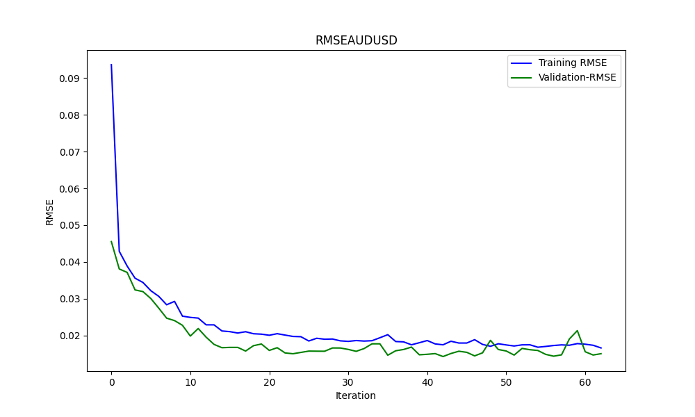
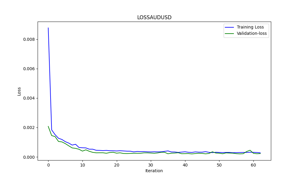
# python libraries
import MetaTrader5 as mt5
import tensorflow as tf
import numpy as np
import pandas as pd
import tf2onnx

# input parameters

inp_history_size = 120

sample_size = 120*20
symbol = "AUDUSD"
optional = "D1"
inp_model_name = str(symbol)+"_"+str(optional)+".onnx" 

if not mt5.initialize():
    print("initialize() failed, error code =",mt5.last_error())
    quit()

# we will save generated onnx-file near the our script to use as resource
from sys import argv
data_path=argv[0]
last_index=data_path.rfind("\\")+1
data_path=data_path[0:last_index]
print("data path to save onnx model",data_path)

# and save to MQL5\Files folder to use as file
terminal_info=mt5.terminal_info()
file_path=terminal_info.data_path+"\\MQL5\\Files\\"
print("file path to save onnx model",file_path)

# set start and end dates for history data
from datetime import timedelta, datetime
#end_date = datetime.now()
end_date = datetime(2023, 1, 1, 0)
start_date = end_date - timedelta(days=inp_history_size*20)

# print start and end dates
print("data start date =",start_date)
print("data end date =",end_date)

# get rates
eurusd_rates = mt5.copy_rates_from(symbol, mt5.TIMEFRAME_D1, end_date, sample_size)

# create dataframe
df = pd.DataFrame(eurusd_rates)

# get close prices only
data = df.filter(['close']).values

# scale data
from sklearn.preprocessing import MinMaxScaler
scaler=MinMaxScaler(feature_range=(0,1))
scaled_data = scaler.fit_transform(data)

# training size is 80% of the data
training_size = int(len(scaled_data)*0.80) 
print("Training_size:",training_size)
train_data_initial = scaled_data[0:training_size,:]
test_data_initial = scaled_data[training_size:,:1]

# split a univariate sequence into samples
def split_sequence(sequence, n_steps):
    X, y = list(), list()
    for i in range(len(sequence)):
       # find the end of this pattern
       end_ix = i + n_steps
       # check if we are beyond the sequence
       if end_ix > len(sequence)-1:
          break
       # gather input and output parts of the pattern
       seq_x, seq_y = sequence[i:end_ix], sequence[end_ix]
       X.append(seq_x)
       y.append(seq_y)
    return np.array(X), np.array(y)

# split into samples
time_step = inp_history_size
x_train, y_train = split_sequence(train_data_initial, time_step)
x_test, y_test = split_sequence(test_data_initial, time_step)

# reshape input to be [samples, time steps, features] which is required for LSTM
x_train =x_train.reshape(x_train.shape[0],x_train.shape[1],1)
x_test = x_test.reshape(x_test.shape[0],x_test.shape[1],1)



# define model
from keras.models import Sequential
from keras.layers import Dense, Activation, Conv1D, MaxPooling1D, Dropout, Flatten, LSTM
from keras.metrics import RootMeanSquaredError as rmse
from tensorflow.keras import callbacks
model = Sequential()
model.add(Conv1D(filters=256, kernel_size=2, activation='relu',padding = 'same',input_shape=(inp_history_size,1)))
model.add(MaxPooling1D(pool_size=2))
model.add(LSTM(100, return_sequences = True))
model.add(Dropout(0.3))
model.add(LSTM(100, return_sequences = False))
model.add(Dropout(0.3))
model.add(Dense(units=1, activation = 'sigmoid'))
model.compile(optimizer='adam', loss= 'mse' , metrics = [rmse()])

# Set up early stopping
early_stopping = callbacks.EarlyStopping(
    monitor='val_loss',
    patience=20,
    restore_best_weights=True,
)

# model training for 300 epochs
history = model.fit(x_train, y_train, epochs = 300 , validation_data = (x_test,y_test), batch_size=32, callbacks=[early_stopping], verbose=2)

# evaluate training data
train_loss, train_rmse = model.evaluate(x_train,y_train, batch_size = 32)
print(f"train_loss={train_loss:.3f}")
print(f"train_rmse={train_rmse:.3f}")

# evaluate testing data
test_loss, test_rmse = model.evaluate(x_test,y_test, batch_size = 32)
print(f"test_loss={test_loss:.3f}")
print(f"test_rmse={test_rmse:.3f}")

# save model to ONNX
output_path = data_path+inp_model_name
onnx_model = tf2onnx.convert.from_keras(model, output_path=output_path)
print(f"saved model to {output_path}")

output_path = file_path+inp_model_name
onnx_model = tf2onnx.convert.from_keras(model, output_path=output_path)
print(f"saved model to {output_path}")

# finish
mt5.shutdown()
#prediction using testing data

#prediction using testing data
test_predict = model.predict(x_test)
print(test_predict)
print("longitud total de la prediccion: ", len(test_predict))
print("longitud total del sample: ", sample_size)

plot_y_test = np.array(y_test).reshape(-1, 1)  # Selecciona solo el último elemento de cada muestra de prueba
plot_y_train = y_train.reshape(-1,1)
train_predict = model.predict(x_train)
#print(plot_y_test)

#calculate metrics
from sklearn import metrics
from sklearn.metrics import r2_score
#transform data to real values
value1=scaler.inverse_transform(plot_y_test)
#print(value1)
# Escala las predicciones inversas al transformarlas a la escala original
value2 = scaler.inverse_transform(test_predict.reshape(-1, 1))
#print(value2)
#calc score
score = np.sqrt(metrics.mean_squared_error(value1,value2))

print("RMSE         : {}".format(score))
print("MSE          :", metrics.mean_squared_error(value1,value2))
print("R2 score     :",metrics.r2_score(value1,value2))


#sumarize model
model.summary()

#Print error
value11=pd.DataFrame(value1)
value22=pd.DataFrame(value2)
#print(value11)
#print(value22)



value111=value11.iloc[:,:]
value222=value22.iloc[:,:]

print("longitud salida (tandas de 1 hora): ",len(value111) )
print("en horas son " + str((len(value111))*60*24)+ " minutos")
print("en horas son " + str(((len(value111)))*60*24/60)+ " horas")
print("en horas son " + str(((len(value111)))*60*24/60/24)+ " dias")


# Calculate error
error = value111 - value222

import matplotlib.pyplot as plt
# Plot error
plt.figure(figsize=(10, 6))
plt.scatter(range(len(error)), error, color='blue', label='Error')
plt.axhline(y=0, color='red', linestyle='--', linewidth=1)  # Línea horizontal en y=0
plt.title('Error de Predicción ' + str(symbol))
plt.xlabel('Índice de la muestra')
plt.ylabel('Error')
plt.legend()
plt.grid(True)
plt.savefig(str(symbol)+str(optional)+'.png') 

rmse_ = format(score)
mse_ = metrics.mean_squared_error(value1,value2)
r2_ = metrics.r2_score(value1,value2)

resultados= [rmse_,mse_,r2_]

# Abre un archivo en modo escritura
with open(str(symbol)+str(optional)+"results.txt", "w") as archivo:
    # Escribe cada resultado en una línea separada
    for resultado in resultados:
        archivo.write(str(resultado) + "\n")

# finish
mt5.shutdown()

#show iteration-rmse graph for training and validation
plt.figure(figsize = (18,10))
plt.plot(history.history['root_mean_squared_error'],label='Training RMSE',color='b')
plt.plot(history.history['val_root_mean_squared_error'],label='Validation-RMSE',color='g')
plt.xlabel("Iteration")
plt.ylabel("RMSE")
plt.title("RMSE" + str(symbol))
plt.legend()
plt.savefig(str(symbol)+str(optional)+'1.png') 

#show iteration-loss graph for training and validation
plt.figure(figsize = (18,10))
plt.plot(history.history['loss'],label='Training Loss',color='b')
plt.plot(history.history['val_loss'],label='Validation-loss',color='g')
plt.xlabel("Iteration")
plt.ylabel("Loss")
plt.title("LOSS" + str(symbol))
plt.legend()
plt.savefig(str(symbol)+str(optional)+'2.png') 

#show actual vs predicted (training) graph
plt.figure(figsize=(18,10))
plt.plot(scaler.inverse_transform(plot_y_train),color = 'b', label = 'Original')
plt.plot(scaler.inverse_transform(train_predict),color='red', label = 'Predicted')
plt.title("Prediction Graph Using Training Data" + str(symbol))
plt.xlabel("Hours")
plt.ylabel("Price")
plt.legend()
plt.savefig(str(symbol)+str(optional)+'3.png') 

#show actual vs predicted (testing) graph
plt.figure(figsize=(18,10))
plt.plot(scaler.inverse_transform(plot_y_test),color = 'b',  label = 'Original')
plt.plot(scaler.inverse_transform(test_predict),color='g', label = 'Predicted')
plt.title("Prediction Graph Using Testing Data" + str(symbol))
plt.xlabel("Hours")
plt.ylabel("Price")
plt.legend()
plt.savefig(str(symbol)+str(optional)+'4.png')

Результатом является модель ONNX. Ниже представлены некоторые графики и значения. Нам понадобятся обе модели из выбранных нами пар корреляции и коинтеграции:

error audusd

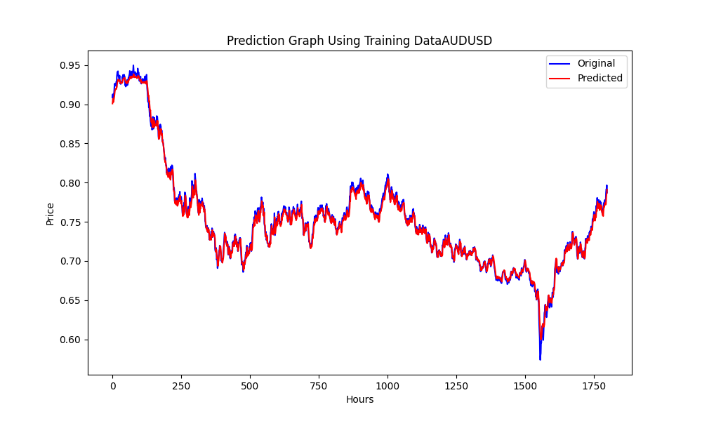
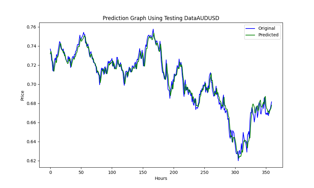
Результаты:

0.005679790676089899
3.226002212419775e-05
0.9670613229880559

Это RMSE, MSE и R2 соответственно.

Тестирование на истории с помощью Python

Вы можете использовать следующий код. Просто измените стратегию и проверьте результаты тестирования на истории:

import MetaTrader5 as mt5
import pandas as pd
from scipy.stats import pearsonr
from statsmodels.tsa.stattools import coint
import numpy as np


# Función para la estrategia de Pairs Trading
def pairs_trading_strategy(data0, data1):
    spread = data0 - data1
    short_entry = np.mean(spread) - 2 * np.std(spread)
    short_exit = np.mean(spread)
    long_entry = np.mean(spread) + 2 * np.std(spread)
    long_exit = np.mean(spread)

    positions = []
    for i in range(len(spread)):
        if spread[i] > long_entry and (not positions or positions[-1][1] != 1):
            positions.append((spread[i], 1))
        elif spread[i] < short_entry and (not positions or positions[-1][1] != -1):
            positions.append((spread[i], -1))
        elif spread[i] < long_exit and positions and positions[-1][1] == 1:
            positions.append((spread[i], 0))
        elif spread[i] > short_exit and positions and positions[-1][1] == -1:
            positions.append((spread[i], 0))

    return positions


# Conectar con MetaTrader 5
if not mt5.initialize():
    print("No se pudo inicializar MT5")
    mt5.shutdown()

# Obtener la lista de símbolos
symbols = mt5.symbols_get()
symbols = [s.name for s in symbols if 'EUR' in s.name or 'USD' in s.name]  # Filtrar símbolos

data = {}
for symbol in symbols:
    rates = mt5.copy_rates_from_pos(symbol, mt5.TIMEFRAME_D1, 0, 365)
    if rates is not None:
        df = pd.DataFrame(rates)
        df['time'] = pd.to_datetime(df['time'], unit='s')  # Convertir a datetime
        df.set_index('time', inplace=True)
        data[symbol] = df['close']

mt5.shutdown()

# Identificar pares cointegrados
cointegrated_pairs = []
for i in range(len(symbols)):
    for j in range(i + 1, len(symbols)):
        if symbols[i] in data and symbols[j] in data:
            common_index = data[symbols[i]].index.intersection(data[symbols[j]].index)
            if len(common_index) > 30:
                corr, _ = pearsonr(data[symbols[i]][common_index], data[symbols[j]][common_index])
                if abs(corr) > 0.8:
                    score, p_value, _ = coint(data[symbols[i]][common_index], data[symbols[j]][common_index])
                    if p_value < 0.05:
                        cointegrated_pairs.append((symbols[i], symbols[j], corr, p_value))

print(cointegrated_pairs)

# Ejecutar estrategia de Pairs Trading para pares cointegrados
for sym1, sym2, _, _ in cointegrated_pairs:
    positions = []
    df0 = data[sym1]
    df1 = data[sym2]

    positions = pairs_trading_strategy(df0.values, df1.values)

    print(f'Backtesting completed for pair: {sym1} - {sym2}')
    print('Positions:', positions)

Тестирование на истории с помощью тестера стратегий MetaTrader 5

Теперь у нас есть модели ONNX и мы можем запустить советник. Я решил использовать простую стратегию. Вы же можете выбрать любую стратегию по вашему желанию. Буду рад, если вы покажете свою стратегию и результаты.

При первом запуске NZDUSD и AUDUSD были коинтегрированы и коррелированы, но на данный момент они не проходят фильтр (коинтеграция меньше 0,05). В учебных целях и для того, чтобы избежать необходимости снова создавать модели ONNX, я продолжу использовать эти два символа.

//+------------------------------------------------------------------+
//|                               Hybrid Arbitrage_Statistic ONNX.mq5|
//|           Copyright 2024, Javier S. Gastón de Iriarte Cabrera. |
//|                      https://www.mql5.com/en/users/jsgaston/news |
//+------------------------------------------------------------------+
#property copyright   "Copyright 2024, Javier S. Gastón de Iriarte Cabrera."
#property link        "https://www.mql5.com/en/users/jsgaston/news"
#property version     "1.00"

#property strict
#include <Trade\Trade.mqh>
input double lotSize = 0.1;
//input double slippage = 3;
input double stopLoss = 1500;
input double takeProfit = 1500;
//input double maxSpreadPoints = 10.0;

#resource "/Files/art/hybrid/NZDUSD_D1.onnx" as uchar ExtModel[]
#resource "/Files/art/hybrid/AUDUSD_D1.onnx" as uchar ExtModel2[]

#define SAMPLE_SIZE 120

string symbol1 = _Symbol;
input string symbol2 = "AUDUSD";
ulong ticket1 = 0;
ulong ticket2 = 0;
input bool isArbitrageActive = true;
CTrade ExtTrade;
double spreads[1000]; // Array para almacenar hasta 1000 spreads
int spreadIndex = 0; // Índice para el próximo spread a almacenar

long     ExtHandle=INVALID_HANDLE;
//int      ExtPredictedClass=-1;
datetime ExtNextBar=0;
datetime ExtNextDay=0;
float    ExtMin=0.0;
float    ExtMax=0.0;


long     ExtHandle2=INVALID_HANDLE;
//int      ExtPredictedClass=-1;
datetime ExtNextBar2=0;
datetime ExtNextDay2=0;
float    ExtMin2=0.0;
float    ExtMax2=0.0;

float predicted=0.0;
float predicted2=0.0;

float   lastPredicted1=0.0;
float   lastPredicted2=0.0;

int Order=0;
//+------------------------------------------------------------------+
//| Expert initialization function                                   |
//+------------------------------------------------------------------+
int OnInit()
  {
   Print("EA de arbitraje ONNX iniciado");

//--- create a model from static buffer
   ExtHandle=OnnxCreateFromBuffer(ExtModel,ONNX_DEFAULT);
   if(ExtHandle==INVALID_HANDLE)
     {
      Print("OnnxCreateFromBuffer error ",GetLastError());
      return(INIT_FAILED);
     }

//--- since not all sizes defined in the input tensor we must set them explicitly
//--- first index - batch size, second index - series size, third index - number of series (only Close)
   const long input_shape[] = {1,SAMPLE_SIZE,1};
   if(!OnnxSetInputShape(ExtHandle,ONNX_DEFAULT,input_shape))
     {
      Print("OnnxSetInputShape error ",GetLastError());
      return(INIT_FAILED);
     }

//--- since not all sizes defined in the output tensor we must set them explicitly
//--- first index - batch size, must match the batch size of the input tensor
//--- second index - number of predicted prices (we only predict Close)
   const long output_shape[] = {1,1};
   if(!OnnxSetOutputShape(ExtHandle,0,output_shape))
     {
      Print("OnnxSetOutputShape error ",GetLastError());
      return(INIT_FAILED);
     }


//--- create a model from static buffer
   ExtHandle2=OnnxCreateFromBuffer(ExtModel2,ONNX_DEFAULT);
   if(ExtHandle2==INVALID_HANDLE)
     {
      Print("OnnxCreateFromBuffer error ",GetLastError());
      return(INIT_FAILED);
     }

//--- since not all sizes defined in the input tensor we must set them explicitly
//--- first index - batch size, second index - series size, third index - number of series (only Close)
   const long input_shape2[] = {1,SAMPLE_SIZE,1};
   if(!OnnxSetInputShape(ExtHandle2,ONNX_DEFAULT,input_shape2))
     {
      Print("OnnxSetInputShape error ",GetLastError());
      return(INIT_FAILED);
     }

//--- since not all sizes defined in the output tensor we must set them explicitly
//--- first index - batch size, must match the batch size of the input tensor
//--- second index - number of predicted prices (we only predict Close)
   const long output_shape2[] = {1,1};
   if(!OnnxSetOutputShape(ExtHandle2,0,output_shape2))
     {
      Print("OnnxSetOutputShape error ",GetLastError());
      return(INIT_FAILED);
     }



   return(INIT_SUCCEEDED);
  }

//+------------------------------------------------------------------+
//| Expert deinitialization function                                 |
//+------------------------------------------------------------------+
void OnDeinit(const int reason)
  {
   if(ExtHandle!=INVALID_HANDLE)
     {
      OnnxRelease(ExtHandle);
      ExtHandle=INVALID_HANDLE;
     }

   if(ExtHandle2!=INVALID_HANDLE)
     {
      OnnxRelease(ExtHandle2);
      ExtHandle2=INVALID_HANDLE;
     }
  }

//+------------------------------------------------------------------+
//| Expert tick function                                             |
//+------------------------------------------------------------------+
void OnTick()
  {
//--- check new day
   if(TimeCurrent()>=ExtNextDay)
     {
      GetMinMax();
      GetMinMax2();
      //--- set next day time
      ExtNextDay=TimeCurrent();
      ExtNextDay-=ExtNextDay%PeriodSeconds(PERIOD_D1);
      ExtNextDay+=PeriodSeconds(PERIOD_D1);
      /*ExtTrade.PositionClose(symbol1);
      ExtTrade.PositionClose(symbol2);
      ticket1 = 0;
      ticket2 = 0;*/
     }

//--- check new bar
   if(TimeCurrent()<ExtNextBar)
     {

      return;
     }
//--- set next bar time
   ExtNextBar=TimeCurrent();
   ExtNextBar-=ExtNextBar%PeriodSeconds();
   ExtNextBar+=PeriodSeconds();
//--- check min and max
   float close=(float)iClose(symbol1,PERIOD_D1,0);
   if(ExtMin>close)
      ExtMin=close;
   if(ExtMax<close)
      ExtMax=close;
   float close2=(float)iClose(symbol2,PERIOD_D1,0);
   if(ExtMin2>close2)
      ExtMin2=close2;
   if(ExtMax2<close2)
      ExtMax2=close2;

   lastPredicted1=predicted;
   lastPredicted2=predicted2;

//--- predict next price
   PredictPrice();
   PredictPrice2();



   if(!isArbitrageActive || ArePositionsOpen())
     {
      Print("Arbitraje inactivo o ya hay posiciones abiertas.");
      return;
     }
   double price1 = SymbolInfoDouble(symbol1, SYMBOL_BID);
   double price2 = SymbolInfoDouble(symbol2, SYMBOL_ASK);
   double currentSpread = MathAbs(price1 - price2);
   Print("current spread ", currentSpread);
   Print("Price1 ",price1);
   Print("Price2 ",price2);
   Print("PricePredicted1 ",predicted);
   Print("PricePredicted2 ",predicted2);
   Print("Last PricePredicted1 ",lastPredicted1);
   Print("Last PricePredicted2 ",lastPredicted2);

   double predictedSpread = MathAbs(predicted - predicted2);
   Print("Predicted spread ", predictedSpread);

   double LastpredictedSpread = MathAbs(lastPredicted1 - lastPredicted2);
   Print("Last Predicted spread ", LastpredictedSpread);

// Almacenar el spread actual en el array y actualizar el índice
   spreads[spreadIndex % 1000] = currentSpread;
   spreadIndex++;

// Verifica si hay suficientes datos para calcular la desviación estándar
   int count = MathMin(spreadIndex, 1000); // Utiliza todos los datos disponibles hasta 1000
   double stdDevSpread = CalculateStdDev(spreads, 0, count);
//Print("StdDevSpread ", stdDevSpread);

// Verifica si el spread es lo suficientemente bajo para el arbitraje
   if(LastpredictedSpread< currentSpread)
     {
      // Inicia el arbitraje si aún no está activo
      if(isArbitrageActive)
        {
         //Print("max spread : ",maxSpreadPoints * _Point);
         double meanSpread = (lastPredicted1 + lastPredicted2) / 2.0;
         Print("mean spread: ",meanSpread);
         double stdDevSpread = CalculateStdDev(spreads, 0, ArraySize(spreads));
         Print("StdDevSpread ", stdDevSpread);
         double shortEntry = meanSpread - 2 * stdDevSpread ;

         double shortExit = meanSpread;
         double longEntry = meanSpread + 2 * stdDevSpread ;

         double longExit = meanSpread;

         Print("Long Entry: ", longEntry, " Short Entry: ", shortEntry);

         // Comprueba si la condición de entrada corta se cumple para el arbitraje
         if(price1 < shortEntry && (ticket1 == 0 || ticket2 == 0))
           {
            Print("Preparando para abrir órdenes");
            Order = 1;


            Print("Error al abrir posiciones de arbitraje: ", GetLastError());
            ticket1 = ExtTrade.PositionOpen(symbol1, ORDER_TYPE_BUY, lotSize, price1, price1 - stopLoss * _Point, price1 + takeProfit * _Point, "Arbitraje");
            ticket2 = ExtTrade.PositionOpen(symbol2, ORDER_TYPE_SELL, lotSize, price2, price2 + stopLoss * _Point, price2 - takeProfit * _Point, "Arbitraje");
            ticket1=0;
            ticket2=0;
           }
         else
            if(price2 < shortEntry && (ticket1 == 0 || ticket2 == 0))
              {
               Print("Preparando para abrir órdenes");
               Order = 2;


               Print("Error al abrir posiciones de arbitraje: ", GetLastError());
               ticket1 = ExtTrade.PositionOpen(symbol1, ORDER_TYPE_SELL, lotSize, price1, price1 + stopLoss * _Point, price1 - takeProfit * _Point, "Arbitraje");
               ticket2 = ExtTrade.PositionOpen(symbol2, ORDER_TYPE_BUY, lotSize, price2, price2 - stopLoss * _Point, price2 + takeProfit * _Point, "Arbitraje");
               ticket1=0;
               ticket2=0;
              }

            else
               if(price1 > longEntry && (ticket1 == 0 || ticket2 == 0))
                 {
                  Print("Preparando para abrir órdenes");
                  Order = 3;


                  Print("Error al abrir posiciones de arbitraje: ", GetLastError());
                  ticket1 = ExtTrade.PositionOpen(symbol1, ORDER_TYPE_SELL, lotSize, price1, price1 + stopLoss * _Point, price1 - takeProfit * _Point, "Arbitraje");
                  ticket2 = ExtTrade.PositionOpen(symbol2, ORDER_TYPE_BUY, lotSize, price2, price2 - stopLoss * _Point, price2 + takeProfit * _Point, "Arbitraje");
                  ticket1=0;
                  ticket2=0;
                 }
               else
                  if(price2 > longEntry && (ticket1 == 0 || ticket2 == 0))
                    {
                     Print("Preparando para abrir órdenes");
                     Order = 4;


                     Print("Error al abrir posiciones de arbitraje: ", GetLastError());

                     ticket1 = ExtTrade.PositionOpen(symbol1, ORDER_TYPE_BUY, lotSize, price1, price1 - stopLoss * _Point, price1 + takeProfit * _Point, "Arbitraje");
                     ticket2 = ExtTrade.PositionOpen(symbol2, ORDER_TYPE_SELL, lotSize, price2, price2 + stopLoss * _Point, price2 - takeProfit * _Point, "Arbitraje");
                     ticket1=0;
                     ticket2=0;
                    }

        }
     }
//+------------------------------------------------------------------+
//|                                                                  |
//+------------------------------------------------------------------+
   double meanSpread = (lastPredicted1 + lastPredicted2) / 2.0;
//Print("mean spread: ",meanSpread);
   double stdDevSpread2 = CalculateStdDev(spreads, 0, ArraySize(spreads));
//Print("StdDevSpread ", stdDevSpread);
   double shortEntry = meanSpread - 2 * stdDevSpread2 ;

   double shortExit = meanSpread;
   double longEntry = meanSpread + 2 * stdDevSpread2 ;

   double longExit = meanSpread;
   if((price2 < longExit && ticket2 != 0 && Order==4) || (price1 > shortExit && ticket1 != 0 && Order==1) || (price2 > shortExit && ticket1 != 0 && Order==2) || (price1 < longExit && ticket2 != 0 && Order==3))
     {
      ExtTrade.PositionClose(ticket1);
      ExtTrade.PositionClose(ticket2);
      ticket1 = 0;
      ticket2 = 0;
      Print("Arbitraje detenido - Cerrando órdenes");
     }

  }

//+------------------------------------------------------------------+
//|                                                                  |
//+------------------------------------------------------------------+
double CalculateStdDev(double &data[], int start, int count)
  {
   double sum = 0;
   double sumSq = 0;
   for(int i = start; i < start + count; i++)
     {
      sum += data[i];
      sumSq += data[i] * data[i];
     }
   double mean = sum / count;
   double variance = (sumSq / count) - (mean * mean);
   return MathSqrt(variance);
  }
//+------------------------------------------------------------------+
//|                                                                  |
//+------------------------------------------------------------------+
bool ArePositionsOpen()
  {
// Check for positions on symbol1
   if(PositionSelect(symbol1) && PositionGetDouble(POSITION_VOLUME) > 0)
      return true;
// Check for positions on symbol2
   if(PositionSelect(symbol2) && PositionGetDouble(POSITION_VOLUME) > 0)
      return true;

   return false;
  }
//+------------------------------------------------------------------+
void PredictPrice(void)
  {
   static vectorf output_data(1);            // vector to get result
   static vectorf x_norm(SAMPLE_SIZE);       // vector for prices normalize

//--- check for normalization possibility
   if(ExtMin>=ExtMax)
     {
      Print("ExtMin>=ExtMax");
      //ExtPredictedClass=-1;
      return;
     }
//--- request last bars
   if(!x_norm.CopyRates(_Symbol,PERIOD_D1,COPY_RATES_CLOSE,1,SAMPLE_SIZE))
     {
      Print("CopyRates ",x_norm.Size());
      //ExtPredictedClass=-1;
      return;
     }
   float last_close=x_norm[SAMPLE_SIZE-1];
//--- normalize prices
   x_norm-=ExtMin;
   x_norm/=(ExtMax-ExtMin);
//--- run the inference
   if(!OnnxRun(ExtHandle,ONNX_NO_CONVERSION,x_norm,output_data))
     {
      Print("OnnxRun");
      //ExtPredictedClass=-1;
      return;
     }
//--- denormalize the price from the output value
   predicted=output_data[0]*(ExtMax-ExtMin)+ExtMin;
//return predicted;
  }
//+------------------------------------------------------------------+
//|                                                                  |
//+------------------------------------------------------------------+
void PredictPrice2(void)
  {
   static vectorf output_data2(1);            // vector to get result
   static vectorf x_norm2(SAMPLE_SIZE);       // vector for prices normalize

//--- check for normalization possibility
   if(ExtMin2>=ExtMax2)
     {
      Print("ExtMin2>=ExtMax2");
      //ExtPredictedClass=-1;
      return;
     }
//--- request last bars
   if(!x_norm2.CopyRates(symbol2,PERIOD_D1,COPY_RATES_CLOSE,1,SAMPLE_SIZE))
     {
      Print("CopyRates ",x_norm2.Size());
      //ExtPredictedClass=-1;
      return;
     }
   float last_close2=x_norm2[SAMPLE_SIZE-1];
//--- normalize prices
   x_norm2-=ExtMin2;
   x_norm2/=(ExtMax2-ExtMin2);
//--- run the inference
   if(!OnnxRun(ExtHandle2,ONNX_NO_CONVERSION,x_norm2,output_data2))
     {
      Print("OnnxRun");
      //ExtPredictedClass=-1;
      return;
     }
//--- denormalize the price from the output value
   predicted2=output_data2[0]*(ExtMax2-ExtMin2)+ExtMin2;
//--- classify predicted price movement
//return predicted2;
  }

//+------------------------------------------------------------------+
//| Get minimal and maximal Close for last 120 days                  |
//+------------------------------------------------------------------+
void GetMinMax(void)
  {
   vectorf close;
   close.CopyRates(_Symbol,PERIOD_D1,COPY_RATES_CLOSE,0,SAMPLE_SIZE);
   ExtMin=close.Min();
   ExtMax=close.Max();
  }

//+------------------------------------------------------------------+
//| Get minimal and maximal Close for last 120 days                  |
//+------------------------------------------------------------------+
void GetMinMax2(void)
  {
   vectorf close2;
   close2.CopyRates(symbol2,PERIOD_D1,COPY_RATES_CLOSE,0,SAMPLE_SIZE);
   ExtMin2=close2.Min();
   ExtMax2=close2.Max();
  }

Это результаты для NZDUSD и AUDUSD M1 с моделями ONNX для однодневного периода времени со стоп-лоссом в 1500 пунктов и тейк-профитом в 1500 пунктов с моделями, которые дают прогноз с первого января 2023 до первого января 2024 года :

nzdusd audusd

nzdusd audusd тестирование на истории

Чтобы выбрать другие пары для сортировки, измените эту строку:

symbols = [s.name for s in symbols if s.name.startswith('EUR') or s.name.startswith('USD') or s.name.endswith('USD')]

Пример 2

Арбитраж очень часто используется в торговле акциями, поэтому мне интересно рассмотреть еще один пример с парами из NASDAQ.

В моем случае я заменил эту строку:

symbols = [s.name for s in symbols if s.name.startswith('EUR') or s.name.startswith('USD') or s.name.endswith('USD')]

следующей:

# Crea un DataFrame con la información completa de los símbolos
symbols_df = pd.DataFrame([{'Symbol': symbol.name, 'Path': symbol.path} for symbol in all_symbols])

# Filtra adicionalmente para obtener solo los CFDs de NASDAQ
# Asumiendo que los CFDs tienen un identificador único en el 'Path'
nasdaq_group4_df = symbols_df[symbols_df['Path'].str.contains('NASDAQ')]

# Filtra aún más para obtener solo los símbolos que NO contienen '.'
nasdaq_group4_df3 = nasdaq_group4_df[nasdaq_group4_df['Symbol'].str.contains('#')]

nasdaq_group4_df2 = nasdaq_group4_df3[~nasdaq_group4_df3['Symbol'].str.contains('\.')]

# Ahora, obtenemos la lista de símbolos filtrados
filtered_symbols = nasdaq_group4_df2['Symbol'].tolist()
# Descargar datos históricos y almacenar en un diccionario
symbols = filtered_symbols

Здесь отсортированы пары:

(Было так много пар, коинтегрированных и коррелированных, что мне пришлось изменить скрипт. Я модифицировал скрипт .py, чтобы вывести его в csv.)

Изменения:

# Filtrar y guardar solo los pares cointegrados con p-valor menor de 0.05 en un archivo CSV
result_df = pd.DataFrame(cointegrated_pairs, columns=['Symbol1', 'Symbol2', 'Correlation', 'Cointegration P-value'])
result_df.to_csv('cointegrated_pairs.csv', index=False)

# Imprimir el total de pares cointegrados
print(f'Total de pares con fuerte correlación y cointegrados: {len(cointegrated_pairs)}')

Это пары, отфильтрованные из NASDAQ (Excel с результатами прилагается).

На данный момент я продолжу работу с моделями Amazon и Netflix, которые прогнозируют период с первого января 2023 года по первое января 2024 года.

#AMZN   #NFLX   0.966605859     0.021683012

Для получения лучших результатов размер выборки был увеличен в три раза.

sample_size = 120*25*3

Вот пример результата:

amzn 0

amzn 1

amzn 2

amzn 3

amzn 4

6.856399020501732
47.010207528337105
0.9395402850007741

nflx 0

nflx 1

nflx 2

nflx 3

nflx 4

25.975755379462548
674.7398675336775
0.9735838717570285

Сто стоп-лоссом 400 и тейк-профитом 800

amzn nflx

amzn nflx тестирование на истории

Затем я настроил стоп-лоссы и тейк-профиты. Вот что мы получили в результате быстрой оптимизации:

Результаты оптимизации

Все скрипты и ONNX с советниками прилагаются к данной статье. Вы можете скачать их и использовать для получения результатов. Вам нужно будет самостоятельно создавать новые ONNX в нужные вам даты (не забудьте изменить даты в обучающих файлах .py), а также даты в тестере стратегий. Пример: модели ONNX для периодов времени D1 и 120*3*25 данных можно использовать максимум в течение года (но на вашем месте я бы создавал их каждую неделю или месяц).

Помните, это всего лишь пример, а не готовый к использованию торговый робот. Вы вряд ли найдете готового робота бесплатно в Интернете.

Заключение

Мы увидели, как использовать корреляцию и коинтеграцию, и создали индикатор коэффициента Пирсона и советник для арбитражной торговли с использованием прогнозов. Лучшие результаты можно получить при использовании правильных пар из фильтра .py. Вы можете точно настроить стоп-уровни, чтобы добиться лучших результатов, а также усложнить стратегию.

Не забудьте сохранить модели ONNX в папке MQL5/Files, индикатор mq5 - в папке Indicator, а советник - в папке Experts.

Перевод с английского произведен MetaQuotes Ltd.
Оригинальная статья: https://www.mql5.com/en/articles/14846

Прикрепленные файлы |

Загрузить ZIP

Pearson.mq5 (7.91 KB)

correlaciin_y_cointegracinn.py (2.02 KB)

ONNX.audusd.D1.120.Training__mod.py (8.16 KB)

ONNX.nzdusd.D1.120.Training__mod.py (8.22 KB)

backtesting.py (2.67 KB)

correlacixn_y_cointegracimn_stocks.py (3.09 KB)

cointegrated_pairs.csv (220.15 KB)

ONNX.amzn.D1.120.Training__mod.py (8.16 KB)

ONNX.nflx.D1.120.Training__mod.py (8.16 KB)

hybrid_statArb_amzn_nflx.mq5 (32.64 KB)

hybrid_statArb_onnx_closeDay.mq5 (29.07 KB)

pAMZN_D1.onnx (884.34 KB)

uNFLX_D1.onnx (884.41 KB)

AUDUSD_D1.onnx (884.37 KB)

NZDUSD_D1.onnx (884.34 KB)

Предупреждение: все права на данные материалы принадлежат MetaQuotes Ltd. Полная или частичная перепечатка запрещена.

Другие статьи автора

Перейти к обсуждению на форуме трейдеров

Машинное обучение и Data Science (Часть 22): Автоэнкодеры для устранения шума и выявления сигналов в трейдинге

В динамичном мире финансовых рынков для успешно торговли важно уметь отделять значимые сигналы от шума. Используя сложную архитектуру нейронных сетей, автоэнкодеры успешно выявляют скрытые закономерности в рыночных данных и преобразуют нечеткие входные данные в полезные идеи. В этой статье мы рассмотрим, как такие нейросети могут помочь принимать торговые решения на современных динамичных рынках.

Алгоритм выбора признаков с использованием энергетического обучения на чистом MQL5

Статья представляет реализацию алгоритма выбора признаков, описанного в научной работе "FREL: Стабильный алгоритм выбора признаков" (FREL: A stable feature selection algorithm). Сам алгоритм называется "Взвешивание признаков как регуляризованное обучение на основе энергии" (Feature weighting as regularized energy based learning).

Возможности Мастера MQL5, которые вам нужно знать (Часть 18): Поиск нейронной архитектуры с использованием собственных векторов

Поиск нейронной архитектуры (Neural Architecture Search), автоматизированный подход к определению идеальных настроек нейронной сети, может стать преимуществом при наличии большого количества вариантов и больших наборов тестовых данных. Здесь мы рассмотрим, как этот подход можно сделать еще более эффективным с помощью парных собственных векторов (Eigen Vectors).

Торговля на разрывах справедливой стоимости (FVG)/дисбалансах шаг за шагом: Подход Smart Money

Пошаговое руководство по созданию и реализации автоматизированного торгового алгоритма на основе разрывов справедливой стоимости (Fair Value Gap, FVG) на языке MQL5. Подробное руководство может быть полезно как новичкам, так и опытным трейдерам.