基于预测的统计套利

MetaTrader 5 — 交易系统 | 19 十一月 2024, 09:52

621

Javier Santiago Gaston De Iriarte Cabrera

概述

统计套利是一种复杂的金融策略，它通过数学模型，利用相关金融工具之间的价格低效性交易获利。该策略通常应用于股票、债券或衍生品，要求深刻理解相关性、协整性以及皮尔逊系数，这些是识别和利用市场机会的关键工具。

在金融领域，相关性用于衡量两种证券之间价格变动的紧密程度，即量化它们之间的关联程度。正相关表明证券的价格通常朝同一方向变动，而负相关则意味着它们的价格朝相反方向变动。交易者会分析这些关系来预测未来的价格走势。

协整是一个更为精细的统计特性，它超越了相关性，通过检验两个或多个时间序列变量的线性组合是否随时间保持稳定来进行分析。简而言之，虽然单个证券可能遵循不同的路径，但它们的相对变动受到某种均衡关系的制约，这种均衡关系使它们倾向于回归。这个概念在成对交易中至关重要，成对交易的目标是识别出历史上价格一起变动，且预期会继续这种趋势的一对股票。

皮尔逊相关系数是一个统计指标，用于计算两个变量之间线性关系的强度和方向。皮尔逊相关系数的值域为-1到1，其中1表示完全正相关，-1表示完全负相关，0表示没有线性关系。在统计套利中，如果两个资产之间的皮尔逊相关系数绝对值较高，这可能意味着存在一个潜在的交易机会，前提是这两个资产的价格关系将回归到长期平均水平。

实施统计套利策略的交易者依赖于算法和高频交易系统来监控和执行交易。这些系统能够处理大量数据，迅速检测出资产价格关系中的异常。该策略假设相关资产的价格将收敛到其历史均值，从而使交易者能够在价格调整中获利。

然而，统计套利的成功不仅取决于复杂的数学模型，还取决于交易者根据不断变化的市场条件解读数据和调整策略的能力。确实，诸如突发经济变动、市场情绪或政治事件等因素，都可能对最稳定的关系造成干扰，从而引发更高层次的风险。

下面用简单的例子来做解释说明

相关性衡量两件事之间的关系。想象一下，你和你最好的朋友总是在星期六一起去看电影。这是一个相关性的例子：当你去电影院时，你的朋友也在那里。如果相关性为正，则意味着当一个增加时，另一个也会增加。如果为负，则一个增加，但另一个减少。如果相关性为0，则意味着两者之间没有联系。

协整是一个统计概念，用于描述两个或多个变量之间虽然短期内可能独立波动，但长期内却存在某种稳定关系的现象。想象一下两个用绳子绑在一起的游泳者：他们可以在泳池中自由游动，但彼此间的距离不会相隔太远。协整表明，尽管这些变量之间会存在暂时的差异，但它们最终总是会回归到共同的长期均衡状态或趋势上。

皮尔逊相关系数用于衡量两个变量之间的线性相关程度。如果相关系数接近+1，则表示一个变量增加时，另一个变量也随之增加，呈现出直接依赖关系。相关系数接近-1时，意味着一个变量增加时，另一个变量减少，呈现出反向关系。相关系数为0时，表示两个变量之间没有线性联系。例如，通过测量温度和冷饮销售量，我们可以使用皮尔逊相关系数来了解这些因素之间的相关性。

总结来说，统计套利是一种复杂但可能带来丰厚回报的交易策略，它融合了经济学、金融学和数学等多个领域的元素。这种策略不仅要求深入理解高级统计概念，还需要具备部署高速算法进行市场分析和执行交易的能力。

计算

要知道哪些交易品种是协整及相关的，可以使用以下.py代码。

import MetaTrader5 as mt5
import pandas as pd
from scipy.stats import pearsonr
from statsmodels.tsa.stattools import coint
import numpy as np

# Connect with MetaTrader 5
if not mt5.initialize():
    print("Failed to initialize MT5")
    mt5.shutdown()

# Get the list of symbols
symbols = mt5.symbols_get()
symbols = [s.name for s in symbols if s.name.startswith('EUR') or s.name.startswith('USD') or s.name.endswith('USD')]  # Filtrar símbolos por ejemplo

# Download historical data and save in dictionary
data = {}
for symbol in symbols:
    rates = mt5.copy_rates_from_pos(symbol, mt5.TIMEFRAME_D1, 0, 365)  # Último año, diario
    if rates is not None:
        df = pd.DataFrame(rates)
        df['time'] = pd.to_datetime(df['time'], unit='s')
        data[symbol] = df.set_index('time')['close']

# Close connection with MT5
mt5.shutdown()

# Calculate the Pearson coefficient and test for cointegration for each pair of symbols
cointegrated_pairs = []
for i in range(len(symbols)):
    for j in range(i + 1, len(symbols)):
        if symbols[i] in data and symbols[j] in data:
            common_index = data[symbols[i]].index.intersection(data[symbols[j]].index)
            if len(common_index) > 30:  # Asegurarse de que hay suficientes puntos de datos
                corr, _ = pearsonr(data[symbols[i]][common_index], data[symbols[j]][common_index])
                if abs(corr) > 0.8:  # Correlación fuerte
                    score, p_value, _ = coint(data[symbols[i]][common_index], data[symbols[j]][common_index])
                    if p_value < 0.05:  # P-valor menor que 0.05
                        cointegrated_pairs.append((symbols[i], symbols[j], corr, p_value))

# Filter and show only cointegrated pairs with p-value less than 0.05
print(f'Total pairs with strong correlation and cointegration: {len(cointegrated_pairs)}')
for sym1, sym2, corr, p_val in cointegrated_pairs:
    print(f'{sym1} - {sym2}: Correlación={corr:.4f}, P-valor de Cointegración={p_val:.4f}')

结果如下：

Total pairs with strong correlation and coitegration: 54
EURUSD - USDBGN: Correlación=-0.9957, P-valor de Cointegración=0.0000
EURUSD - USDHRK: Correlación=-0.9972, P-valor de Cointegración=0.0000
GBPUSD - USDPLN: Correlación=-0.8633, P-valor de Cointegración=0.0406
GBPUSD - GBXUSD: Correlación=0.9998, P-valor de Cointegración=0.0000
GBPUSD - EURSGD: Correlación=0.8061, P-valor de Cointegración=0.0191
USDCHF - EURCHF: Correlación=0.8324, P-valor de Cointegración=0.0356
USDJPY - EURDKK: Correlación=0.8338, P-valor de Cointegración=0.0200
USDJPY - USDTHB: Correlación=0.9012, P-valor de Cointegración=0.0330
AUDUSD - USDCNH: Correlación=-0.8074, P-valor de Cointegración=0.0390
EURCHF - USDKES: Correlación=-0.9104, P-valor de Cointegración=0.0048
EURJPY - EURRON: Correlación=0.8177, P-valor de Cointegración=0.0333
EURJPY - USDCOP: Correlación=-0.9361, P-valor de Cointegración=0.0125
EURJPY - USDLAK: Correlación=0.9508, P-valor de Cointegración=0.0410
EURJPY - EURDKK: Correlación=0.8525, P-valor de Cointegración=0.0136
EURJPY - EURMXN: Correlación=-0.8785, P-valor de Cointegración=0.0172
EURJPY - USDTRY: Correlación=0.9564, P-valor de Cointegración=0.0102
EURNZD - NZDUSD: Correlación=-0.8505, P-valor de Cointegración=0.0455
EURNZD - EURDKK: Correlación=0.8242, P-valor de Cointegración=0.0017
EURCZK - USDCLP: Correlación=0.9655, P-valor de Cointegración=0.0001
USDCLP - USDCZK: Correlación=0.8972, P-valor de Cointegración=0.0147
USDCLP - USDARS: Correlación=0.8077, P-valor de Cointegración=0.0231
USDCLP - USDIDR: Correlación=0.8569, P-valor de Cointegración=0.0423
USDCLP - USDNGN: Correlación=0.8468, P-valor de Cointegración=0.0436
USDCLP - USDVND: Correlación=0.9021, P-valor de Cointegración=0.0194
USDCZK - USDIDR: Correlación=0.9005, P-valor de Cointegración=0.0086
USDCZK - USDVND: Correlación=0.8306, P-valor de Cointegración=0.0195
USDMXN - USDCOP: Correlación=0.8686, P-valor de Cointegración=0.0286
USDMXN - EURMXN: Correlación=0.9522, P-valor de Cointegración=0.0328
NZDUSD - USDSGD: Correlación=-0.8145, P-valor de Cointegración=0.0097
NZDUSD - USDTHB: Correlación=-0.8094, P-valor de Cointegración=0.0255
ADAUSD - KSMUSD: Correlación=0.9429, P-valor de Cointegración=0.0071
ALGUSD - LNKUSD: Correlación=0.8038, P-valor de Cointegración=0.0454
ATMUSD - MTCUSD: Correlación=0.9423, P-valor de Cointegración=0.0146
BTCUSD - SOLUSD: Correlación=0.9736, P-valor de Cointegración=0.0112
DGEUSD - GLDUSD: Correlación=0.8933, P-valor de Cointegración=0.0136
DGEUSD - USDGHS: Correlación=0.8562, P-valor de Cointegración=0.0101
EOSUSD - UNIUSD: Correlación=0.8176, P-valor de Cointegración=0.0051
ETCUSD - ETHUSD: Correlación=0.9745, P-valor de Cointegración=0.0009
ETCUSD - SOLUSD: Correlación=0.9206, P-valor de Cointegración=0.0093
ETCUSD - UNIUSD: Correlación=0.9236, P-valor de Cointegración=0.0249
ETHUSD - SOLUSD: Correlación=0.9430, P-valor de Cointegración=0.0074
UNIUSD - USDNGN: Correlación=0.8074, P-valor de Cointegración=0.0195
EURNOK - USDNOK: Correlación=0.9065, P-valor de Cointegración=0.0430
EURRON - USDCOP: Correlación=-0.8010, P-valor de Cointegración=0.0097
EURRON - USDCRC: Correlación=-0.8015, P-valor de Cointegración=0.0159
EURRON - USDLAK: Correlación=0.8364, P-valor de Cointegración=0.0349
GBXUSD - EURSGD: Correlación=0.8067, P-valor de Cointegración=0.0180
USDARS - USDVND: Correlación=0.8093, P-valor de Cointegración=0.0268
USDBGN - USDHRK: Correlación=0.9944, P-valor de Cointegración=0.0000
USDCOP - USDTRY: Correlación=-0.9548, P-valor de Cointegración=0.0160
USDCRC - EURDKK: Correlación=-0.8519, P-valor de Cointegración=0.0153
USDHRK - USDDKK: Correlación=0.9954, P-valor de Cointegración=0.0000
USDIDR - USDVND: Correlación=0.8196, P-valor de Cointegración=0.0417
USDSEK - USDSGD: Correlación=0.8346, P-valor de Cointegración=0.0264

因此，这些货币对已被过滤掉。

为了用MetaTrader 5检查这些值，我们有了这个指标（Pearson.mq5）：

//+------------------------------------------------------------------+
//|                                             PearsonIndicator.mq5 |
//|                    Copyright Javier S. Gastón de Iriarte Cabrera |
//|                                       https://www.mql5.com/en/users/jsgaston/news |
//+------------------------------------------------------------------+
#property copyright "Javier S. Gastón de Iriarte Cabrera"
#property link      "https://www.mql5.com/en/users/jsgaston/news/"
#property version   "1.00"
#property indicator_separate_window
#property indicator_buffers 1
#property indicator_color1 Red

input string Symbol2 = "GBPUSD";       // Second financial instrument
input int BarsBack = 100;              // Number of bars to include in correlation calculation

double CorrelationBuffer[];

//+------------------------------------------------------------------+
//| Custom indicator initialization function                         |
//+------------------------------------------------------------------+
int OnInit()
  {
   SetIndexBuffer(0, CorrelationBuffer, INDICATOR_DATA);
   PlotIndexSetInteger(0, PLOT_DRAW_TYPE, DRAW_LINE);
   PlotIndexSetString(0, PLOT_LABEL, "Pearson Correlation");
   IndicatorSetString(INDICATOR_SHORTNAME, "Pearson Correlation (" + Symbol() + " & " + Symbol2 + ")");
   return INIT_SUCCEEDED;
  }

//+------------------------------------------------------------------+
//| Custom indicator iteration function                              |
//+------------------------------------------------------------------+
int OnCalculate(const int rates_total,
                const int prev_calculated,
                const datetime &time[],
                const double &open[],
                const double &high[],
                const double &low[],
                const double &close[],
                const long &tick_volume[],
                const long &volume[],
                const int &spread[])
  {
   if (rates_total < BarsBack) return 0; // Ensure enough bars are present

   double prices1[], prices2[];
   ArrayResize(prices1, BarsBack);
   ArrayResize(prices2, BarsBack);

   // Copy historical data for primary symbol
   if (CopyClose(Symbol(), PERIOD_CURRENT, 0, BarsBack, prices1) <= 0)
      {
       Print("Error copying prices for ", Symbol());
       return 0;
      }
   // Copy historical data for secondary symbol
   if (CopyClose(Symbol2, PERIOD_CURRENT, 0, BarsBack, prices2) <= 0)
      {
       Print("Error copying prices for ", Symbol2);
       return 0;
      }

   // Calculate Pearson correlation for the entire buffer
   double correlation = CalculatePearsonCorrelation(prices1, prices2);
   Print("Pearson correlation: ", correlation);

   // Fill the buffer for the indicator
   for (int i = BarsBack; i < rates_total; i++)
     {
      CorrelationBuffer[i] = correlation;  // Update the buffer correctly
     }

   return(rates_total);
  }

//+------------------------------------------------------------------+
//| Calculate Pearson correlation coefficient                        |
//+------------------------------------------------------------------+
double CalculatePearsonCorrelation(double &prices1[], double &prices2[])
  {
   int length = BarsBack;
   double mean1 = 0, mean2 = 0;
   double sum1 = 0, sum2 = 0, sumProd = 0, stdev1 = 0, stdev2 = 0;

   for (int i = 0; i < length; i++)
     {
      mean1 += prices1[i];
      mean2 += prices2[i];
     }
   mean1 /= length;
   mean2 /= length;

   for (int i = 0; i < length; i++)
     {
      double dev1 = prices1[i] - mean1;
      double dev2 = prices2[i] - mean2;
      sum1 += dev1 * dev1;
      sum2 += dev2 * dev2;
      sumProd += dev1 * dev2;
     }
   stdev1 = sqrt(sum1);
   stdev2 = sqrt(sum2);

   if (stdev1 == 0 || stdev2 == 0) return 0; // Avoid division by zero
   return sumProd / (stdev1 * stdev2);
  }
//+------------------------------------------------------------------+

结果显示：

皮尔逊

建立ONNX模型

一旦我们知道了哪些货币对是相互关联且协整的，并且在mql5中检查了皮尔逊相关系数之后，我们就可以构建一个ONNX模型来研究这两对货币对过去的表现。

# python libraries
import MetaTrader5 as mt5
import tensorflow as tf
import numpy as np
import pandas as pd
import tf2onnx

# input parameters

inp_history_size = 120

sample_size = 120*20
symbol = "AUDUSD"
optional = "D1"
inp_model_name = str(symbol)+"_"+str(optional)+".onnx" 

if not mt5.initialize():
    print("initialize() failed, error code =",mt5.last_error())
    quit()

# we will save generated onnx-file near the our script to use as resource
from sys import argv
data_path=argv[0]
last_index=data_path.rfind("\\")+1
data_path=data_path[0:last_index]
print("data path to save onnx model",data_path)

# and save to MQL5\Files folder to use as file
terminal_info=mt5.terminal_info()
file_path=terminal_info.data_path+"\\MQL5\\Files\\"
print("file path to save onnx model",file_path)

# set start and end dates for history data
from datetime import timedelta, datetime
#end_date = datetime.now()
end_date = datetime(2023, 1, 1, 0)
start_date = end_date - timedelta(days=inp_history_size*20)

# print start and end dates
print("data start date =",start_date)
print("data end date =",end_date)

# get rates
eurusd_rates = mt5.copy_rates_from(symbol, mt5.TIMEFRAME_D1, end_date, sample_size)

# create dataframe
df = pd.DataFrame(eurusd_rates)

# get close prices only
data = df.filter(['close']).values

# scale data
from sklearn.preprocessing import MinMaxScaler
scaler=MinMaxScaler(feature_range=(0,1))
scaled_data = scaler.fit_transform(data)

# training size is 80% of the data
training_size = int(len(scaled_data)*0.80) 
print("Training_size:",training_size)
train_data_initial = scaled_data[0:training_size,:]
test_data_initial = scaled_data[training_size:,:1]

# split a univariate sequence into samples
def split_sequence(sequence, n_steps):
    X, y = list(), list()
    for i in range(len(sequence)):
       # find the end of this pattern
       end_ix = i + n_steps
       # check if we are beyond the sequence
       if end_ix > len(sequence)-1:
          break
       # gather input and output parts of the pattern
       seq_x, seq_y = sequence[i:end_ix], sequence[end_ix]
       X.append(seq_x)
       y.append(seq_y)
    return np.array(X), np.array(y)

# split into samples
time_step = inp_history_size
x_train, y_train = split_sequence(train_data_initial, time_step)
x_test, y_test = split_sequence(test_data_initial, time_step)

# reshape input to be [samples, time steps, features] which is required for LSTM
x_train =x_train.reshape(x_train.shape[0],x_train.shape[1],1)
x_test = x_test.reshape(x_test.shape[0],x_test.shape[1],1)



# define model
from keras.models import Sequential
from keras.layers import Dense, Activation, Conv1D, MaxPooling1D, Dropout, Flatten, LSTM
from keras.metrics import RootMeanSquaredError as rmse
from tensorflow.keras import callbacks
model = Sequential()
model.add(Conv1D(filters=256, kernel_size=2, activation='relu',padding = 'same',input_shape=(inp_history_size,1)))
model.add(MaxPooling1D(pool_size=2))
model.add(LSTM(100, return_sequences = True))
model.add(Dropout(0.3))
model.add(LSTM(100, return_sequences = False))
model.add(Dropout(0.3))
model.add(Dense(units=1, activation = 'sigmoid'))
model.compile(optimizer='adam', loss= 'mse' , metrics = [rmse()])

# Set up early stopping
early_stopping = callbacks.EarlyStopping(
    monitor='val_loss',
    patience=20,
    restore_best_weights=True,
)

# model training for 300 epochs
history = model.fit(x_train, y_train, epochs = 300 , validation_data = (x_test,y_test), batch_size=32, callbacks=[early_stopping], verbose=2)

# evaluate training data
train_loss, train_rmse = model.evaluate(x_train,y_train, batch_size = 32)
print(f"train_loss={train_loss:.3f}")
print(f"train_rmse={train_rmse:.3f}")

# evaluate testing data
test_loss, test_rmse = model.evaluate(x_test,y_test, batch_size = 32)
print(f"test_loss={test_loss:.3f}")
print(f"test_rmse={test_rmse:.3f}")

# save model to ONNX
output_path = data_path+inp_model_name
onnx_model = tf2onnx.convert.from_keras(model, output_path=output_path)
print(f"saved model to {output_path}")

output_path = file_path+inp_model_name
onnx_model = tf2onnx.convert.from_keras(model, output_path=output_path)
print(f"saved model to {output_path}")

# finish
mt5.shutdown()
#prediction using testing data

#prediction using testing data
test_predict = model.predict(x_test)
print(test_predict)
print("longitud total de la prediccion: ", len(test_predict))
print("longitud total del sample: ", sample_size)

plot_y_test = np.array(y_test).reshape(-1, 1)  # Selecciona solo el último elemento de cada muestra de prueba
plot_y_train = y_train.reshape(-1,1)
train_predict = model.predict(x_train)
#print(plot_y_test)

#calculate metrics
from sklearn import metrics
from sklearn.metrics import r2_score
#transform data to real values
value1=scaler.inverse_transform(plot_y_test)
#print(value1)
# Escala las predicciones inversas al transformarlas a la escala original
value2 = scaler.inverse_transform(test_predict.reshape(-1, 1))
#print(value2)
#calc score
score = np.sqrt(metrics.mean_squared_error(value1,value2))

print("RMSE         : {}".format(score))
print("MSE          :", metrics.mean_squared_error(value1,value2))
print("R2 score     :",metrics.r2_score(value1,value2))


#sumarize model
model.summary()

#Print error
value11=pd.DataFrame(value1)
value22=pd.DataFrame(value2)
#print(value11)
#print(value22)



value111=value11.iloc[:,:]
value222=value22.iloc[:,:]

print("longitud salida (tandas de 1 hora): ",len(value111) )
print("en horas son " + str((len(value111))*60*24)+ " minutos")
print("en horas son " + str(((len(value111)))*60*24/60)+ " horas")
print("en horas son " + str(((len(value111)))*60*24/60/24)+ " dias")


# Calculate error
error = value111 - value222

import matplotlib.pyplot as plt
# Plot error
plt.figure(figsize=(10, 6))
plt.scatter(range(len(error)), error, color='blue', label='Error')
plt.axhline(y=0, color='red', linestyle='--', linewidth=1)  # Línea horizontal en y=0
plt.title('Error de Predicción ' + str(symbol))
plt.xlabel('Índice de la muestra')
plt.ylabel('Error')
plt.legend()
plt.grid(True)
plt.savefig(str(symbol)+str(optional)+'.png') 

rmse_ = format(score)
mse_ = metrics.mean_squared_error(value1,value2)
r2_ = metrics.r2_score(value1,value2)

resultados= [rmse_,mse_,r2_]

# Abre un archivo en modo escritura
with open(str(symbol)+str(optional)+"results.txt", "w") as archivo:
    # Escribe cada resultado en una línea separada
    for resultado in resultados:
        archivo.write(str(resultado) + "\n")

# finish
mt5.shutdown()

#show iteration-rmse graph for training and validation
plt.figure(figsize = (18,10))
plt.plot(history.history['root_mean_squared_error'],label='Training RMSE',color='b')
plt.plot(history.history['val_root_mean_squared_error'],label='Validation-RMSE',color='g')
plt.xlabel("Iteration")
plt.ylabel("RMSE")
plt.title("RMSE" + str(symbol))
plt.legend()
plt.savefig(str(symbol)+str(optional)+'1.png') 

#show iteration-loss graph for training and validation
plt.figure(figsize = (18,10))
plt.plot(history.history['loss'],label='Training Loss',color='b')
plt.plot(history.history['val_loss'],label='Validation-loss',color='g')
plt.xlabel("Iteration")
plt.ylabel("Loss")
plt.title("LOSS" + str(symbol))
plt.legend()
plt.savefig(str(symbol)+str(optional)+'2.png') 

#show actual vs predicted (training) graph
plt.figure(figsize=(18,10))
plt.plot(scaler.inverse_transform(plot_y_train),color = 'b', label = 'Original')
plt.plot(scaler.inverse_transform(train_predict),color='red', label = 'Predicted')
plt.title("Prediction Graph Using Training Data" + str(symbol))
plt.xlabel("Hours")
plt.ylabel("Price")
plt.legend()
plt.savefig(str(symbol)+str(optional)+'3.png') 

#show actual vs predicted (testing) graph
plt.figure(figsize=(18,10))
plt.plot(scaler.inverse_transform(plot_y_test),color = 'b',  label = 'Original')
plt.plot(scaler.inverse_transform(test_predict),color='g', label = 'Predicted')
plt.title("Prediction Graph Using Testing Data" + str(symbol))
plt.xlabel("Hours")
plt.ylabel("Price")
plt.legend()
plt.savefig(str(symbol)+str(optional)+'4.png')

此.py生成ONNX模型和一些图表以及数值，如下所示。我们需要从我们选择的相关性和协整对中选择两个模型：

错误audusd

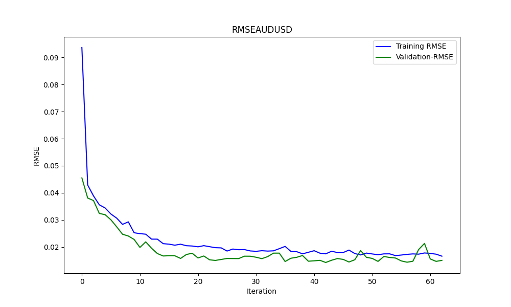
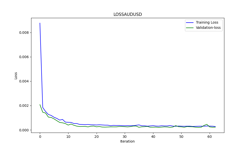
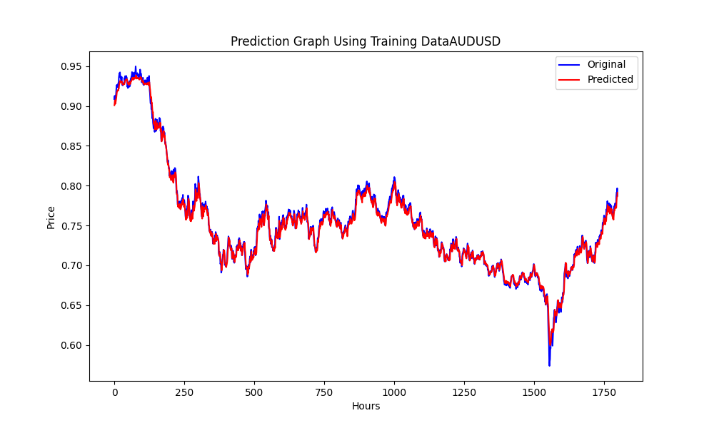
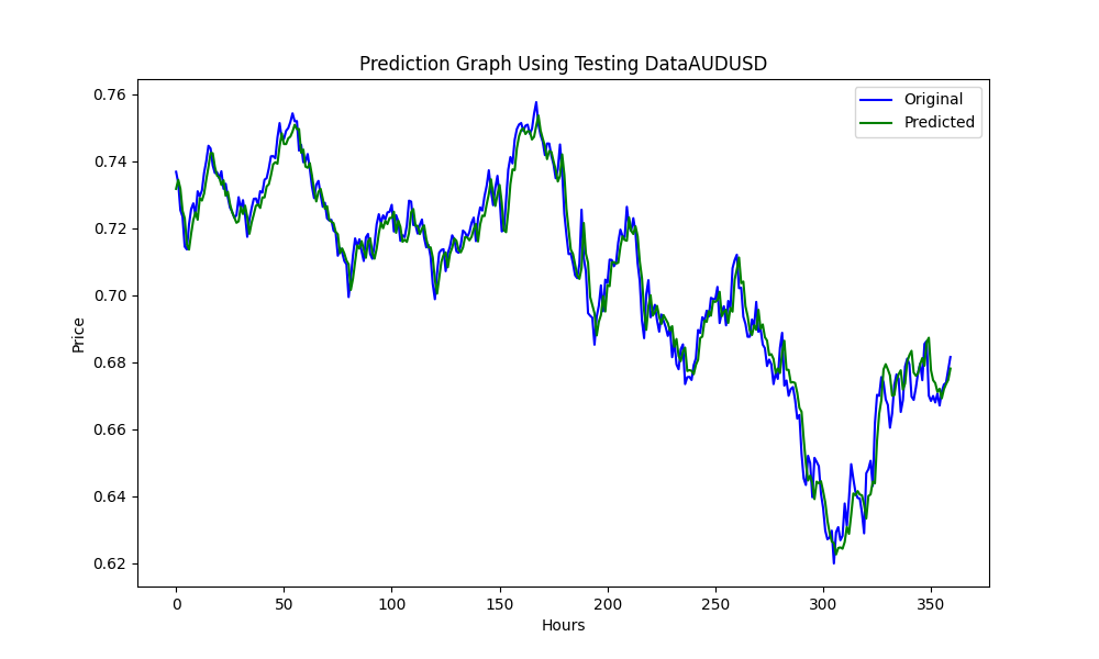
结果如下

0.005679790676089899
3.226002212419775e-05
0.9670613229880559

这些分别是RMSE、MSE和R2。

使用Python进行反向测试

您可以使用以下.py代码。只需更改策略并检查回溯测试的结果：

import MetaTrader5 as mt5
import pandas as pd
from scipy.stats import pearsonr
from statsmodels.tsa.stattools import coint
import numpy as np


# Función para la estrategia de Pairs Trading
def pairs_trading_strategy(data0, data1):
    spread = data0 - data1
    short_entry = np.mean(spread) - 2 * np.std(spread)
    short_exit = np.mean(spread)
    long_entry = np.mean(spread) + 2 * np.std(spread)
    long_exit = np.mean(spread)

    positions = []
    for i in range(len(spread)):
        if spread[i] > long_entry and (not positions or positions[-1][1] != 1):
            positions.append((spread[i], 1))
        elif spread[i] < short_entry and (not positions or positions[-1][1] != -1):
            positions.append((spread[i], -1))
        elif spread[i] < long_exit and positions and positions[-1][1] == 1:
            positions.append((spread[i], 0))
        elif spread[i] > short_exit and positions and positions[-1][1] == -1:
            positions.append((spread[i], 0))

    return positions


# Conectar con MetaTrader 5
if not mt5.initialize():
    print("No se pudo inicializar MT5")
    mt5.shutdown()

# Obtener la lista de símbolos
symbols = mt5.symbols_get()
symbols = [s.name for s in symbols if 'EUR' in s.name or 'USD' in s.name]  # Filtrar símbolos

data = {}
for symbol in symbols:
    rates = mt5.copy_rates_from_pos(symbol, mt5.TIMEFRAME_D1, 0, 365)
    if rates is not None:
        df = pd.DataFrame(rates)
        df['time'] = pd.to_datetime(df['time'], unit='s')  # Convertir a datetime
        df.set_index('time', inplace=True)
        data[symbol] = df['close']

mt5.shutdown()

# Identificar pares cointegrados
cointegrated_pairs = []
for i in range(len(symbols)):
    for j in range(i + 1, len(symbols)):
        if symbols[i] in data and symbols[j] in data:
            common_index = data[symbols[i]].index.intersection(data[symbols[j]].index)
            if len(common_index) > 30:
                corr, _ = pearsonr(data[symbols[i]][common_index], data[symbols[j]][common_index])
                if abs(corr) > 0.8:
                    score, p_value, _ = coint(data[symbols[i]][common_index], data[symbols[j]][common_index])
                    if p_value < 0.05:
                        cointegrated_pairs.append((symbols[i], symbols[j], corr, p_value))

print(cointegrated_pairs)

# Ejecutar estrategia de Pairs Trading para pares cointegrados
for sym1, sym2, _, _ in cointegrated_pairs:
    positions = []
    df0 = data[sym1]
    df1 = data[sym2]

    positions = pairs_trading_strategy(df0.values, df1.values)

    print(f'Backtesting completed for pair: {sym1} - {sym2}')
    print('Positions:', positions)

使用MT5策略测试器进行反向测试

一旦我们有了ONNX模型，就可以运行EA了。我选择了一个简单的策略，但你可以选择任何你想要的或需要的策略。如果你愿意展示你的策略及其结果，我也很欢迎。

当我第一次自行操作时，NZDUSD和AUDUSD是协整且相关的，但此刻它们没有通过筛选（协整度小于0.05）。为了教学目的，也为了避免再次创建ONNX模型，我将继续使用这两个交易品类。

//+------------------------------------------------------------------+
//|                               Hybrid Arbitrage_Statistic ONNX.mq5|
//|           Copyright 2024, Javier S. Gastón de Iriarte Cabrera. |
//|                      https://www.mql5.com/en/users/jsgaston/news |
//+------------------------------------------------------------------+
#property copyright   "Copyright 2024, Javier S. Gastón de Iriarte Cabrera."
#property link        "https://www.mql5.com/en/users/jsgaston/news"
#property version     "1.00"

#property strict
#include <Trade\Trade.mqh>
input double lotSize = 0.1;
//input double slippage = 3;
input double stopLoss = 1500;
input double takeProfit = 1500;
//input double maxSpreadPoints = 10.0;

#resource "/Files/art/hybrid/NZDUSD_D1.onnx" as uchar ExtModel[]
#resource "/Files/art/hybrid/AUDUSD_D1.onnx" as uchar ExtModel2[]

#define SAMPLE_SIZE 120

string symbol1 = _Symbol;
input string symbol2 = "AUDUSD";
ulong ticket1 = 0;
ulong ticket2 = 0;
input bool isArbitrageActive = true;
CTrade ExtTrade;
double spreads[1000]; // Array para almacenar hasta 1000 spreads
int spreadIndex = 0; // Índice para el próximo spread a almacenar

long     ExtHandle=INVALID_HANDLE;
//int      ExtPredictedClass=-1;
datetime ExtNextBar=0;
datetime ExtNextDay=0;
float    ExtMin=0.0;
float    ExtMax=0.0;


long     ExtHandle2=INVALID_HANDLE;
//int      ExtPredictedClass=-1;
datetime ExtNextBar2=0;
datetime ExtNextDay2=0;
float    ExtMin2=0.0;
float    ExtMax2=0.0;

float predicted=0.0;
float predicted2=0.0;

float   lastPredicted1=0.0;
float   lastPredicted2=0.0;

int Order=0;
//+------------------------------------------------------------------+
//| Expert initialization function                                   |
//+------------------------------------------------------------------+
int OnInit()
  {
   Print("EA de arbitraje ONNX iniciado");

//--- create a model from static buffer
   ExtHandle=OnnxCreateFromBuffer(ExtModel,ONNX_DEFAULT);
   if(ExtHandle==INVALID_HANDLE)
     {
      Print("OnnxCreateFromBuffer error ",GetLastError());
      return(INIT_FAILED);
     }

//--- since not all sizes defined in the input tensor we must set them explicitly
//--- first index - batch size, second index - series size, third index - number of series (only Close)
   const long input_shape[] = {1,SAMPLE_SIZE,1};
   if(!OnnxSetInputShape(ExtHandle,ONNX_DEFAULT,input_shape))
     {
      Print("OnnxSetInputShape error ",GetLastError());
      return(INIT_FAILED);
     }

//--- since not all sizes defined in the output tensor we must set them explicitly
//--- first index - batch size, must match the batch size of the input tensor
//--- second index - number of predicted prices (we only predict Close)
   const long output_shape[] = {1,1};
   if(!OnnxSetOutputShape(ExtHandle,0,output_shape))
     {
      Print("OnnxSetOutputShape error ",GetLastError());
      return(INIT_FAILED);
     }


//--- create a model from static buffer
   ExtHandle2=OnnxCreateFromBuffer(ExtModel2,ONNX_DEFAULT);
   if(ExtHandle2==INVALID_HANDLE)
     {
      Print("OnnxCreateFromBuffer error ",GetLastError());
      return(INIT_FAILED);
     }

//--- since not all sizes defined in the input tensor we must set them explicitly
//--- first index - batch size, second index - series size, third index - number of series (only Close)
   const long input_shape2[] = {1,SAMPLE_SIZE,1};
   if(!OnnxSetInputShape(ExtHandle2,ONNX_DEFAULT,input_shape2))
     {
      Print("OnnxSetInputShape error ",GetLastError());
      return(INIT_FAILED);
     }

//--- since not all sizes defined in the output tensor we must set them explicitly
//--- first index - batch size, must match the batch size of the input tensor
//--- second index - number of predicted prices (we only predict Close)
   const long output_shape2[] = {1,1};
   if(!OnnxSetOutputShape(ExtHandle2,0,output_shape2))
     {
      Print("OnnxSetOutputShape error ",GetLastError());
      return(INIT_FAILED);
     }



   return(INIT_SUCCEEDED);
  }

//+------------------------------------------------------------------+
//| Expert deinitialization function                                 |
//+------------------------------------------------------------------+
void OnDeinit(const int reason)
  {
   if(ExtHandle!=INVALID_HANDLE)
     {
      OnnxRelease(ExtHandle);
      ExtHandle=INVALID_HANDLE;
     }

   if(ExtHandle2!=INVALID_HANDLE)
     {
      OnnxRelease(ExtHandle2);
      ExtHandle2=INVALID_HANDLE;
     }
  }

//+------------------------------------------------------------------+
//| Expert tick function                                             |
//+------------------------------------------------------------------+
void OnTick()
  {
//--- check new day
   if(TimeCurrent()>=ExtNextDay)
     {
      GetMinMax();
      GetMinMax2();
      //--- set next day time
      ExtNextDay=TimeCurrent();
      ExtNextDay-=ExtNextDay%PeriodSeconds(PERIOD_D1);
      ExtNextDay+=PeriodSeconds(PERIOD_D1);
      /*ExtTrade.PositionClose(symbol1);
      ExtTrade.PositionClose(symbol2);
      ticket1 = 0;
      ticket2 = 0;*/
     }

//--- check new bar
   if(TimeCurrent()<ExtNextBar)
     {

      return;
     }
//--- set next bar time
   ExtNextBar=TimeCurrent();
   ExtNextBar-=ExtNextBar%PeriodSeconds();
   ExtNextBar+=PeriodSeconds();
//--- check min and max
   float close=(float)iClose(symbol1,PERIOD_D1,0);
   if(ExtMin>close)
      ExtMin=close;
   if(ExtMax<close)
      ExtMax=close;
   float close2=(float)iClose(symbol2,PERIOD_D1,0);
   if(ExtMin2>close2)
      ExtMin2=close2;
   if(ExtMax2<close2)
      ExtMax2=close2;

   lastPredicted1=predicted;
   lastPredicted2=predicted2;

//--- predict next price
   PredictPrice();
   PredictPrice2();



   if(!isArbitrageActive || ArePositionsOpen())
     {
      Print("Arbitraje inactivo o ya hay posiciones abiertas.");
      return;
     }
   double price1 = SymbolInfoDouble(symbol1, SYMBOL_BID);
   double price2 = SymbolInfoDouble(symbol2, SYMBOL_ASK);
   double currentSpread = MathAbs(price1 - price2);
   Print("current spread ", currentSpread);
   Print("Price1 ",price1);
   Print("Price2 ",price2);
   Print("PricePredicted1 ",predicted);
   Print("PricePredicted2 ",predicted2);
   Print("Last PricePredicted1 ",lastPredicted1);
   Print("Last PricePredicted2 ",lastPredicted2);

   double predictedSpread = MathAbs(predicted - predicted2);
   Print("Predicted spread ", predictedSpread);

   double LastpredictedSpread = MathAbs(lastPredicted1 - lastPredicted2);
   Print("Last Predicted spread ", LastpredictedSpread);

// Almacenar el spread actual en el array y actualizar el índice
   spreads[spreadIndex % 1000] = currentSpread;
   spreadIndex++;

// Verifica si hay suficientes datos para calcular la desviación estándar
   int count = MathMin(spreadIndex, 1000); // Utiliza todos los datos disponibles hasta 1000
   double stdDevSpread = CalculateStdDev(spreads, 0, count);
//Print("StdDevSpread ", stdDevSpread);

// Verifica si el spread es lo suficientemente bajo para el arbitraje
   if(LastpredictedSpread< currentSpread)
     {
      // Inicia el arbitraje si aún no está activo
      if(isArbitrageActive)
        {
         //Print("max spread : ",maxSpreadPoints * _Point);
         double meanSpread = (lastPredicted1 + lastPredicted2) / 2.0;
         Print("mean spread: ",meanSpread);
         double stdDevSpread = CalculateStdDev(spreads, 0, ArraySize(spreads));
         Print("StdDevSpread ", stdDevSpread);
         double shortEntry = meanSpread - 2 * stdDevSpread ;

         double shortExit = meanSpread;
         double longEntry = meanSpread + 2 * stdDevSpread ;

         double longExit = meanSpread;

         Print("Long Entry: ", longEntry, " Short Entry: ", shortEntry);

         // Comprueba si la condición de entrada corta se cumple para el arbitraje
         if(price1 < shortEntry && (ticket1 == 0 || ticket2 == 0))
           {
            Print("Preparando para abrir órdenes");
            Order = 1;


            Print("Error al abrir posiciones de arbitraje: ", GetLastError());
            ticket1 = ExtTrade.PositionOpen(symbol1, ORDER_TYPE_BUY, lotSize, price1, price1 - stopLoss * _Point, price1 + takeProfit * _Point, "Arbitraje");
            ticket2 = ExtTrade.PositionOpen(symbol2, ORDER_TYPE_SELL, lotSize, price2, price2 + stopLoss * _Point, price2 - takeProfit * _Point, "Arbitraje");
            ticket1=0;
            ticket2=0;
           }
         else
            if(price2 < shortEntry && (ticket1 == 0 || ticket2 == 0))
              {
               Print("Preparando para abrir órdenes");
               Order = 2;


               Print("Error al abrir posiciones de arbitraje: ", GetLastError());
               ticket1 = ExtTrade.PositionOpen(symbol1, ORDER_TYPE_SELL, lotSize, price1, price1 + stopLoss * _Point, price1 - takeProfit * _Point, "Arbitraje");
               ticket2 = ExtTrade.PositionOpen(symbol2, ORDER_TYPE_BUY, lotSize, price2, price2 - stopLoss * _Point, price2 + takeProfit * _Point, "Arbitraje");
               ticket1=0;
               ticket2=0;
              }

            else
               if(price1 > longEntry && (ticket1 == 0 || ticket2 == 0))
                 {
                  Print("Preparando para abrir órdenes");
                  Order = 3;


                  Print("Error al abrir posiciones de arbitraje: ", GetLastError());
                  ticket1 = ExtTrade.PositionOpen(symbol1, ORDER_TYPE_SELL, lotSize, price1, price1 + stopLoss * _Point, price1 - takeProfit * _Point, "Arbitraje");
                  ticket2 = ExtTrade.PositionOpen(symbol2, ORDER_TYPE_BUY, lotSize, price2, price2 - stopLoss * _Point, price2 + takeProfit * _Point, "Arbitraje");
                  ticket1=0;
                  ticket2=0;
                 }
               else
                  if(price2 > longEntry && (ticket1 == 0 || ticket2 == 0))
                    {
                     Print("Preparando para abrir órdenes");
                     Order = 4;


                     Print("Error al abrir posiciones de arbitraje: ", GetLastError());

                     ticket1 = ExtTrade.PositionOpen(symbol1, ORDER_TYPE_BUY, lotSize, price1, price1 - stopLoss * _Point, price1 + takeProfit * _Point, "Arbitraje");
                     ticket2 = ExtTrade.PositionOpen(symbol2, ORDER_TYPE_SELL, lotSize, price2, price2 + stopLoss * _Point, price2 - takeProfit * _Point, "Arbitraje");
                     ticket1=0;
                     ticket2=0;
                    }

        }
     }
//+------------------------------------------------------------------+
//|                                                                  |
//+------------------------------------------------------------------+
   double meanSpread = (lastPredicted1 + lastPredicted2) / 2.0;
//Print("mean spread: ",meanSpread);
   double stdDevSpread2 = CalculateStdDev(spreads, 0, ArraySize(spreads));
//Print("StdDevSpread ", stdDevSpread);
   double shortEntry = meanSpread - 2 * stdDevSpread2 ;

   double shortExit = meanSpread;
   double longEntry = meanSpread + 2 * stdDevSpread2 ;

   double longExit = meanSpread;
   if((price2 < longExit && ticket2 != 0 && Order==4) || (price1 > shortExit && ticket1 != 0 && Order==1) || (price2 > shortExit && ticket1 != 0 && Order==2) || (price1 < longExit && ticket2 != 0 && Order==3))
     {
      ExtTrade.PositionClose(ticket1);
      ExtTrade.PositionClose(ticket2);
      ticket1 = 0;
      ticket2 = 0;
      Print("Arbitraje detenido - Cerrando órdenes");
     }

  }

//+------------------------------------------------------------------+
//|                                                                  |
//+------------------------------------------------------------------+
double CalculateStdDev(double &data[], int start, int count)
  {
   double sum = 0;
   double sumSq = 0;
   for(int i = start; i < start + count; i++)
     {
      sum += data[i];
      sumSq += data[i] * data[i];
     }
   double mean = sum / count;
   double variance = (sumSq / count) - (mean * mean);
   return MathSqrt(variance);
  }
//+------------------------------------------------------------------+
//|                                                                  |
//+------------------------------------------------------------------+
bool ArePositionsOpen()
  {
// Check for positions on symbol1
   if(PositionSelect(symbol1) && PositionGetDouble(POSITION_VOLUME) > 0)
      return true;
// Check for positions on symbol2
   if(PositionSelect(symbol2) && PositionGetDouble(POSITION_VOLUME) > 0)
      return true;

   return false;
  }
//+------------------------------------------------------------------+
void PredictPrice(void)
  {
   static vectorf output_data(1);            // vector to get result
   static vectorf x_norm(SAMPLE_SIZE);       // vector for prices normalize

//--- check for normalization possibility
   if(ExtMin>=ExtMax)
     {
      Print("ExtMin>=ExtMax");
      //ExtPredictedClass=-1;
      return;
     }
//--- request last bars
   if(!x_norm.CopyRates(_Symbol,PERIOD_D1,COPY_RATES_CLOSE,1,SAMPLE_SIZE))
     {
      Print("CopyRates ",x_norm.Size());
      //ExtPredictedClass=-1;
      return;
     }
   float last_close=x_norm[SAMPLE_SIZE-1];
//--- normalize prices
   x_norm-=ExtMin;
   x_norm/=(ExtMax-ExtMin);
//--- run the inference
   if(!OnnxRun(ExtHandle,ONNX_NO_CONVERSION,x_norm,output_data))
     {
      Print("OnnxRun");
      //ExtPredictedClass=-1;
      return;
     }
//--- denormalize the price from the output value
   predicted=output_data[0]*(ExtMax-ExtMin)+ExtMin;
//return predicted;
  }
//+------------------------------------------------------------------+
//|                                                                  |
//+------------------------------------------------------------------+
void PredictPrice2(void)
  {
   static vectorf output_data2(1);            // vector to get result
   static vectorf x_norm2(SAMPLE_SIZE);       // vector for prices normalize

//--- check for normalization possibility
   if(ExtMin2>=ExtMax2)
     {
      Print("ExtMin2>=ExtMax2");
      //ExtPredictedClass=-1;
      return;
     }
//--- request last bars
   if(!x_norm2.CopyRates(symbol2,PERIOD_D1,COPY_RATES_CLOSE,1,SAMPLE_SIZE))
     {
      Print("CopyRates ",x_norm2.Size());
      //ExtPredictedClass=-1;
      return;
     }
   float last_close2=x_norm2[SAMPLE_SIZE-1];
//--- normalize prices
   x_norm2-=ExtMin2;
   x_norm2/=(ExtMax2-ExtMin2);
//--- run the inference
   if(!OnnxRun(ExtHandle2,ONNX_NO_CONVERSION,x_norm2,output_data2))
     {
      Print("OnnxRun");
      //ExtPredictedClass=-1;
      return;
     }
//--- denormalize the price from the output value
   predicted2=output_data2[0]*(ExtMax2-ExtMin2)+ExtMin2;
//--- classify predicted price movement
//return predicted2;
  }

//+------------------------------------------------------------------+
//| Get minimal and maximal Close for last 120 days                  |
//+------------------------------------------------------------------+
void GetMinMax(void)
  {
   vectorf close;
   close.CopyRates(_Symbol,PERIOD_D1,COPY_RATES_CLOSE,0,SAMPLE_SIZE);
   ExtMin=close.Min();
   ExtMax=close.Max();
  }

//+------------------------------------------------------------------+
//| Get minimal and maximal Close for last 120 days                  |
//+------------------------------------------------------------------+
void GetMinMax2(void)
  {
   vectorf close2;
   close2.CopyRates(symbol2,PERIOD_D1,COPY_RATES_CLOSE,0,SAMPLE_SIZE);
   ExtMin2=close2.Min();
   ExtMax2=close2.Max();
  }

这些是NZDUSD与AUDUSD在1分钟时段内的结果，而ONNX模型为1天时段，SL为1500点，TP为1500点，模型预测时间为2023年1月1日至2024年1月初：

nzdusd audusd

nzdusd audusd back-testing

如需重新选择其它对，请更改此行：

symbols = [s.name for s in symbols if s.name.startswith('EUR') or s.name.startswith('USD') or s.name.endswith('USD')]

案例研究2

套利在股票交易领域很常用，这就是为什么我觉得用纳斯达克的对冲组合来做另一个例子会很有意思。

对我而言，我修改了这一行：

symbols = [s.name for s in symbols if s.name.startswith('EUR') or s.name.startswith('USD') or s.name.endswith('USD')]

对此：

# Crea un DataFrame con la información completa de los símbolos
symbols_df = pd.DataFrame([{'Symbol': symbol.name, 'Path': symbol.path} for symbol in all_symbols])

# Filtra adicionalmente para obtener solo los CFDs de NASDAQ
# Asumiendo que los CFDs tienen un identificador único en el 'Path'
nasdaq_group4_df = symbols_df[symbols_df['Path'].str.contains('NASDAQ')]

# Filtra aún más para obtener solo los símbolos que NO contienen '.'
nasdaq_group4_df3 = nasdaq_group4_df[nasdaq_group4_df['Symbol'].str.contains('#')]

nasdaq_group4_df2 = nasdaq_group4_df3[~nasdaq_group4_df3['Symbol'].str.contains('\.')]

# Ahora, obtenemos la lista de símbolos filtrados
filtered_symbols = nasdaq_group4_df2['Symbol'].tolist()
# Descargar datos históricos y almacenar en un diccionario
symbols = filtered_symbols

这就是配对过滤之处：

（在那里，有太多的配对是协整和相关的，我不得不改变剧本。我修改了.py脚本，以csv格式打印出来。）

更改：

# Filtrar y guardar solo los pares cointegrados con p-valor menor de 0.05 en un archivo CSV
result_df = pd.DataFrame(cointegrated_pairs, columns=['Symbol1', 'Symbol2', 'Correlation', 'Cointegration P-value'])
result_df.to_csv('cointegrated_pairs.csv', index=False)

# Imprimir el total de pares cointegrados
print(f'Total de pares con fuerte correlación y cointegrados: {len(cointegrated_pairs)}')

您已经从纳斯达克中筛选出了这些股票对（附上了包含结果的Excel文件）。

从现在开始，我将继续使用Amazon和Netflix这两个股票对，同时使用预测从2023年1月1日至2024年1月1日的模型。

#AMZN   #NFLX   0.966605859     0.021683012

为了获得更好的结果，将样本量扩大了三倍。

sample_size = 120*25*3

结果如下：

amzn 0

amzn 1

amzn 2

amzn 3

amzn 4

6.856399020501732
47.010207528337105
0.9395402850007741

nflx 0

nflx 1

nflx 2

nflx 3

nflx 4

25.975755379462548
674.7398675336775
0.9735838717570285

止损400止盈800

amzn nflx

amzn和nflx反向测试

之后我对止损和止盈做出了微调。这就是我们通过快速优化得到的结果：

优化结果

所有脚本、ONNX模型以及与EA相关的内容都已附在本文中。您可以根据需要下载，系统且科学地运用它们来获得您的分析结果。您需要根据自己需要的日期来创建新的ONNX模型（记得在训练用的.py文件中更改日期），并同时在策略测试器中更改日期。例如：针对D1时间段的ONNX模型，以及最多使用120*3*25条数据，这些数据可以覆盖一年多的时间（但如果我是您，我会选择每周或每月创建一次模型）。

请记住，这只是一个策略及示例，并不是一个即插即用的交易EA，而且您可能永远无法通过互联网免费找到一个像这样的EA。