
Estrategia de trading del SP500 en MQL5 para principiantes

Introducción
En este artículo analizaremos cómo podemos desarrollar una estrategia comercial inteligente para operar con el índice Standard & Poor's 500 (S&P 500) utilizando MQL5. Nuestro debate demostrará cómo aprovechar la flexibilidad de MQL5 para crear un asesor experto dinámico que se base en una combinación de inteligencia artificial y análisis técnico. Nuestro razonamiento es que confiar únicamente en la IA puede llevar a estrategias inestables; sin embargo, al guiar la IA con los principios probados del análisis técnico, podemos lograr un enfoque más confiable. Esta estrategia híbrida tiene como objetivo descubrir patrones ocultos dentro de las grandes cantidades de datos disponibles en nuestras terminales MetaTrader 5, aprovechando las fortalezas de la IA, el análisis tradicional y el lenguaje MQL5 para mejorar el rendimiento comercial y la toma de decisiones.
Después de leer este artículo, usted obtendrá:
- Buenos principios de programación para MQL5
- Información sobre cómo los comerciantes pueden analizar fácilmente grandes conjuntos de datos de múltiples símbolos simultáneamente utilizando comandos de álgebra lineal en la API MQL5.
- Técnicas para descubrir patrones ocultos en datos de mercado que no son inmediatamente evidentes.
Historia: ¿Qué es el Standard & Poor's 500?
El S&P 500, creado en 1957, es un índice de referencia crucial que refleja el desempeño general de la economía estadounidense. A lo largo de los años, se han añadido y eliminado numerosas empresas al índice, lo que refleja la naturaleza dinámica del mercado. Entre los miembros más antiguos se encuentran General Electric, J.P. Morgan y Goldman Sachs han mantenido sus posiciones en el índice desde su creación.
El S&P 500 representa el valor promedio de las 500 empresas más grandes de los Estados Unidos de América. Al valor de cada empresa se le asigna un peso en función de su capitalización de mercado. Por lo tanto, el S&P 500 también puede considerarse un índice ponderado por capitalización de mercado de las 500 empresas más grandes que cotizan en bolsa en el mundo.
Hoy en día, empresas pioneras como Tesla y Nvidia han redefinido el punto de referencia desde su fundación. En la actualidad, la mayor parte del peso del S&P 500 está en manos de grandes empresas tecnológicas, entre las que se incluyen Google, Apple y Microsoft, entre los gigantes antes mencionados. Estos titanes tecnológicos han transformado el panorama del índice, reflejando el cambio de la economía hacia la tecnología y la innovación.
Descripción general de nuestra estrategia comercial
Una lista de las empresas incluidas en el índice es fácilmente accesible en Internet. Podemos aprovechar nuestra comprensión de cómo se compone el índice para ayudarnos a crear una estrategia comercial. Seleccionaremos un puñado de las empresas más grandes del índice y utilizaremos el precio respectivo de cada empresa como entrada para un modelo de IA que predecirá el precio de cierre del índice basándose en nuestra muestra de empresas que tienen pesos proporcionalmente grandes. Nuestro deseo es desarrollar una estrategia que combine la IA con técnicas confiables y probadas a lo largo del tiempo.
Nuestro sistema de análisis técnico empleará principios de seguimiento de tendencias para generar señales comerciales. Necesitamos incorporar varios indicadores clave:
- El índice de canal de productos básicos (Commodity Channel Index, CCI) sera nuestro indicador de volumen. Sólo queremos ingresar a operaciones que estén respaldadas por volumen.
- El índice de fuerza relativa (Relative Strength Index, RSI) y el rango de porcentaje de Williams (Williams Percent Range, WPR) para medir la presión de compra o venta en el mercado.
- Una media móvil (MA) como nuestro indicador de confirmación final.
El índice de canal de productos básicos (CCI) gira alrededor de 0. Una lectura superior a 0 sugiere un volumen fuerte para una oportunidad de compra, mientras que una lectura inferior a 0 indica un volumen de soporte para la venta. Requerimos alineación con otros indicadores para la confirmación comercial, mejorando nuestras posibilidades de encontrar configuraciones de alta probabilidad.
Por lo tanto, para que podamos comprar:
- La lectura del CCI debe ser mayor que 0.
- La lectura del RSI debe ser mayor que 50.
- La lectura de WPR debe ser mayor que -50.
- MA debe estar por debajo del precio de cierre.
Y a la inversa para que vendamos:
- La lectura del CCI debe ser menor que 0.
- La lectura del RSI debe ser inferior a 50.
- La lectura de WPR debe ser menor que -50.
- MA debe estar por encima del precio de cierre.
Por otro lado, para construir nuestro sistema de IA, primero necesitamos obtener los precios históricos de 12 acciones de gran capitalización de mercado incluidas en el S&P 500 y los precios de cierre del S&P 500. Estos serán nuestros datos de entrenamiento que usaremos para construir nuestro modelo de regresión lineal múltiple para pronosticar los precios futuros del índice.
A partir de ahí, el sistema de IA utilizará la regresión de mínimos cuadrados ordinarios para pronosticar el valor de cierre del S&P 500.

Figura 1: Nuestro modelo verá el S&P 500 como el resultado de una colección de estas acciones.
Una vez que tengamos los datos listos, podemos estimar los parámetros del modelo para nuestro modelo de regresión lineal utilizando la siguiente fórmula.
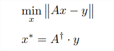
Figura 2: La ecuación anterior demuestra una de las muchas formas posibles de estimar los parámetros de un modelo de regresión lineal múltiple.
La expresión "Ax - y" rodeada de dos líneas verticales se conoce como la norma L2 de un vector, que se pronuncia "ell 2". En el lenguaje cotidiano, cuando preguntamos "¿cuánto mide?" sobre objetos físicos, hablamos de su tamaño o magnitud. De manera similar, cuando preguntamos "qué tan grande" es un vector, nos referimos a su norma. Un vector es esencialmente una lista de números. Si bien existen diferentes tipos de normas, la norma L1 y la norma L2 son las más comunes. Hoy nos centraremos en la norma L2, que se calcula como la raíz cuadrada de la suma de los valores al cuadrado dentro del vector.
En este contexto:
- La matriz "A" representa los datos de entrada, que consisten en los valores de cierre de 12 acciones diferentes.
- El símbolo "x" denota los valores de los coeficientes para nuestro modelo de regresión lineal múltiple, con un coeficiente por acción.
- El producto "Ax" representa nuestras predicciones para el precio futuro del índice S&P 500 basadas en nuestros datos de entrenamiento.
- La notación "y" simboliza el vector de precios de cierre reales que queríamos predecir durante el entrenamiento.
En esencia, la primera ecuación nos dice que estamos buscando valores de x que minimicen la norma L2 de Ax - y. En otras palabras, buscamos los valores de x que minimicen nuestro error de predicción al pronosticar el precio de cierre del S&P 500.
La segunda ecuación revela que los valores de x que logran el error mínimo se pueden encontrar multiplicando la pseudoinversa de A por los datos de salida (y) de nuestro conjunto de entrenamiento. La operación pseudoinversa se implementa convenientemente en MQL5.
Podemos encontrar eficientemente la solución pseudo-inversa en MQL5 con solo unas pocas líneas de código.
Implementación: Estrategia de trading del SP500
Empezando
Primero debemos definir las entradas para nuestro Asesor Experto. Necesitamos entradas que permitan al usuario cambiar los períodos de nuestros indicadores técnicos.
//+------------------------------------------------------------------+
//|                                            SP500 Strategy EA.mq5 |
//|                                  Copyright 2024, MetaQuotes Ltd. |
//|                                             https://www.mql5.com |
//+------------------------------------------------------------------+
#property copyright "Gamuchirai Zororo Ndawana"
#property link      "https://www.mql5.com"
#property version   "1.00"
/*
The goal of this application is to implement a strategy to trade the SP500 based
on the performance of a sample of stocks that hold proportionally large weights in the index and classical technical analysis.

We will use the following stocks:
1)Microsoft
2)Apple
3)Google
4)Meta
5)Visa
6)JPMorgan
7)Nvidia
8)Tesla
9)Johnsons N Johnsons
10)Home Depot
11)Proctor & Gamble
12)Master Card

A strategy that relies solely on AI  may prove to be unstable.
We want to use a combination of AI guided by trading strategies that have been trusted over time.

Our AI will be a linear system mapping the price of each stock to the closing price of the index.
Recall that financial time series data can be very noisy. Using simpler models may be beneficial.
We will attempt to find linear coefficients using ordinary least squares.
We will use the pseudo inverse solution to find our model parameters.

Our technical analysis will be based on trend following principles:
1)We must observe increasing volume backing a trade before we enter.
2)We want 2 confirmation indicators, RSI and WPR, confirming the trend.
3)We want price to break above the previous week high or low.
4)We want price above or below our MA before we trade.

Our goal is to find an optimal combination of statistical insight,
and classical technical analysis to hopefully build a strategy with an edge.

Gamuchirai Zororo Ndawana
Selebi Phikwe
Botswana
Monday 8 July 2024 21:03
*/
//Inputs
//How far ahead into the future should we forecast?
input int look_ahead = 10;
//Our moving average period
input int ma_period = 120;
//Our RSI period
input int rsi_period = 10;
//Our WPR period
input int wpr_period = 30;
//Our CCI period
input int cci_period = 40;
//How big should our lot sizes be?
int input  lot_multiple = 20;
A continuación necesitamos importar nuestra biblioteca comercial para que podamos administrar nuestras posiciones.
//Libraries
//Trade class
#include <Trade/Trade.mqh>
CTrade Trade;
Continuando, necesitamos definir las variables globales que se utilizan en todo nuestro programa.
//Global variables
//Smallest lot size
double minimum_volume;
//Ask
double ask_price;
//Bid
double bid_price;
//How much data should we fetch?
int fetch = 20;
//Determine the starting date for our inputs
int inupt_start;
//Determine the starting date for our outputs
int output_start;
//Which symbols are we going to use to forecast the SP500 close?
string desired_symbols[] = {"MSFT","AAPL","NVDA","GOOG","TSLA","META","JPM","JNJ","V","PG","HD","MA"};
//Define our input matrix
matrix input_matrix = matrix::Ones(fetch,(ArraySize(desired_symbols))-1);
//Define our output matrix, our output matrix has one column
matrix output_matrix = matrix::Ones(fetch,1);
//A vector to store the initial values of each column
vector initiall_input_values = vector::Ones((ArraySize(desired_symbols)));
//A variable to store the initial value of the output
double initiall_output_value = 0.0;
//Defining the matrix that will store our model parameters
matrix b;
//Define our target symbol
string target_symbol = "US_500";
//A vector to temporarily store the historic closing price of each stock
vector symbol_history = vector::Zeros(fetch);
//A flag to let us know when our model is ready
bool model_initialized = false;
//A flag to let us know if the training process has started
bool model_being_trained = false;
//Our model's prediction
double model_forecast = 0;
//Handlers for our technical indicators
int cci_handler,rsi_handler,wpr_handler,ma_handler;
//Buffers for our technical indicator values
double cci_buffer[],rsi_buffer[],wpr_buffer[],ma_buffer[];
Ahora que hemos llegado hasta aquí, debemos configurar nuestros indicadores técnicos en el controlador de inicialización.
//+------------------------------------------------------------------+
//| Expert initialization function                                   |
//+------------------------------------------------------------------+
int OnInit()
  {
//---
//Let's setup our technical indicators
   rsi_handler = iRSI(target_symbol,PERIOD_CURRENT,rsi_period,PRICE_CLOSE);
   ma_handler = iMA(target_symbol,PERIOD_CURRENT,ma_period,0,MODE_EMA,PRICE_CLOSE);
   wpr_handler = iWPR(target_symbol,PERIOD_CURRENT,wpr_period);
   cci_handler = iCCI(target_symbol,PERIOD_CURRENT,cci_period,PRICE_CLOSE);
//Get market data
   minimum_volume = SymbolInfoDouble(_Symbol,SYMBOL_VOLUME_MIN);
//---
   return(INIT_SUCCEEDED);
  }
Necesitamos funciones auxiliares. Inicialmente, definimos un procedimiento para inicializar nuestro modelo de regresión lineal múltiple. Nuestro procedimiento de ajuste comienza colocando una bandera para indicar que nuestro modelo está en entrenamiento. Las funciones adicionales manejan tareas como la recuperación de datos de entrenamiento y el ajuste del modelo. Al dividir nuestro código en funciones más pequeñas, evitaremos escribir las mismas líneas de código varias veces.
//+------------------------------------------------------------------+
//This function defines the procedure for fitting our model
void model_initialize(void)
  {
   /*
   Our function will run the initialization procedure as follows:
   1)Update the training flag to show that the model has been trained
   2)Fetch the necessary input and output data
   3)Preprocess the data, normalization and scaling etc.
   4)Fit the model
   5)Update the flags to show that the model has been trained.
Desde allí nuestra aplicación tendrá la capacidad de comenzar a operar.
   */
//First let us set our flag to denote that the model is being trained
   model_being_trained = true;
//Defining the input start time and the output start time
//Remember the input data should not contain the most recent bars
//The most recent bars must only be included in the output start time
//The input data should be older than the output data.
   inupt_start = 1+look_ahead;
   output_start = 1;
//Fetch the input data
   fetch_input_data(inupt_start,fetch);
//Fetch the output data
   fetch_output_data(output_start,fetch);
//Prepare the data
   prepare_data(0);
//Fit our model
   fit_linear_model();
//The model is ready
   model_ready();
  }
Ahora, procedemos a definir la función responsable de obtener nuestros datos de entrada. Nuestra matriz de entrada incluirá una columna de unos en la primera columna para representar el punto de intersección o el precio de cierre promedio del S&P 500 cuando todos los valores de las acciones son cero. Aunque este escenario no tiene sentido en el mundo financiero, ya que si todos los valores de las acciones fueran 0, el precio de cierre del S&P 500 también sería 0.
Dejando esto de lado, nuestro procedimiento para obtener datos de entrada es sencillo:
- Inicializa la matriz de entrada llena de unos.
- Reformar la matriz
- Complete el valor de cierre de cada acción, comenzando desde la segunda columna
- Asegúrese de que la primera columna esté llena de unos.
//This function will get our input data ready
void fetch_input_data(int f_input_start,int f_fetch)
  {
   /*
      To get the input data ready we will to cycle through the symbols available and copy the requested
      amount of data to the globally scoped input matrix.
      Our function parameters are:
      1)f_input_start: this is where we should get our input data, for the current data pass 0 and only fetch 1.
      2)f_fetch: this is how much data should be fetched and copied into the input matrix.
   */
   Print("Preparing to fetch input data");
//Let's observe the original state of our input matrix
   Print("We will reset the input matrix before fetching the data we need: ");
   input_matrix = matrix::Ones(f_fetch,(ArraySize(desired_symbols))-1);
   Print(input_matrix);
//We need to reshape our matrix
   input_matrix.Reshape(f_fetch,13);
//Filling the input matrix
//Then we need to prepare our input matrix.
//The first column must be full of 1's because it represents the intercept.
//Therefore we will skip 0, and start filling input values from column 1. This is not a mistake.
   for(int i=1; i <= ArraySize(desired_symbols);i++)
     {
      //Copy the input data we need
      symbol_history.CopyRates(desired_symbols[i-1],PERIOD_CURRENT,COPY_RATES_CLOSE,f_input_start,f_fetch);
      //Insert the input data into our input matrix
      input_matrix.Col(symbol_history,i);
     }
//Ensure that the first column is full of ones for our intercept
   vector intercept = vector::Ones(f_fetch);
   input_matrix.Col(intercept,0);
//Let us see what our input matrix looks like now.
   Print("Final state of our input matrix: ");
   Print(input_matrix);
  }
Nuestro procedimiento para obtener datos de salida será más o menos el mismo que usamos para obtener datos de entrada.
//This function will get our output data ready
void fetch_output_data(int f_output_start, int f_fetch)
  {
   /*
      This function will fetch our output data for training our model and copy it into
      our globally defined output matrix. The model has only 2 parameters:
      1)f_output_start: where should we start copying our output data
      2)f_fetch: amount of data to copy
   */
   Print("Preparing to fetch output data");
//Let's observe the original state of our output matrix
   Print("Ressetting output matrix before fetching the data we need: ");
//Reset the output matrix
   output_matrix = matrix::Ones(f_fetch,1);
   Print(output_matrix);
//We need to reshape our matrix
   output_matrix.Reshape(f_fetch,1);
//Output data
//Copy the output data we need
   symbol_history.CopyRates(target_symbol,PERIOD_CURRENT,COPY_RATES_CLOSE,f_output_start,f_fetch);
//Insert the output data into our input matrix
   output_matrix.Col(symbol_history,0);
//Let us see what our input matrix looks like now.
   Print("Final state of our output matrix: ");
   Print(output_matrix);
  }
Antes de ajustar nuestro modelo, necesitamos estandarizar y escalar nuestros datos. Este es un paso importante porque hace que sea más fácil para nuestra aplicación aprender las relaciones ocultas en las tasas de cambio.
Tenga en cuenta que nuestro procedimiento de ajuste tiene dos fases distintas: en la fase 1, cuando se entrena el modelo por primera vez, necesitamos almacenar los valores que usamos para escalar cada columna en un vector. Cada columna se dividirá por el primer valor que contenga, lo que significa que el primer valor de cada columna será uno.
A partir de ese momento, si observamos cualquier valor menor a uno en esa columna, entonces el precio bajó, y valores mayores a uno indican que el precio aumentó. Si observamos una lectura de 0,72, entonces el precio cayó un 28% y si observamos un valor de 1,017, entonces el precio aumentó un 1,7%.
Solo debemos almacenar el valor inicial de cada columna una vez, de ahí en adelante todas las entradas futuras deben dividirse por la misma cantidad para garantizar la consistencia.
//This function will normalize our input data so that our model can learn better
//We will also scale our output so that it shows the growth in price
void prepare_data(int f_flag)
  {
   /*
      This function is responsible for normalizing our inputs and outputs.
      We want to first store the initial value of each column.
      Then we will divide each column by its first value, so that the first value in each column is one.
      The above steps are performed only once, when the model is initialized. All subsequent inputs will
      simply be divided by the initial values of that column.
   */

   Print("Normalizing and scaling the data");
//This part of the procedure should only be performed once
   if(f_flag == 0)
     {
      Print("Preparing to normalize the data for training the model");
      //Normalizing the inputs
      //Store the initial value of each column
      for(int i=0;i<ArraySize(desired_symbols);i++)
        {
         //First we store the initial value of each column
         initiall_input_values[i] = input_matrix[0][i+1];
         //Now temporarily copy the column, so that we can normalize the entire column at once
         vector temp_vector = input_matrix.Col(i+1);
         //Now divide that entire column by its initial value, if done correctly the first value of each column should be 1
         temp_vector = temp_vector / initiall_input_values[i];
         //Now reinsert the normalized column
         input_matrix.Col(temp_vector,i+1);
        }
      //Print the initial input values
      Print("Our initial input values for each column ");
      Print(initiall_input_values);

      //Scale the output
      //Store the initial output value
      initiall_output_value = output_matrix[0][0];
      //Make a temporary copy of the entire output column
      vector temp_vector_output = output_matrix.Col(0);
      //Divide the entire column by its initial value, so that the first value in the column is one
      //This means that any time the value is less than 1, price fell
      //And every time the value is greater than 1, price rose.
      //A value of 1.023... means price increased by 2.3%
      //A value of 0.8732.. would mean price fell by 22.67%
      temp_vector_output = temp_vector_output / initiall_output_value;
      //Reinsert the column back into the output matrix
      output_matrix.Col(temp_vector_output,0);
      //Shpw the scaled data
      Print("Data has been normlised and the output has been scaled:");
      Print("Input matrix: ");
      Print(input_matrix);
      Print("Output matrix: ");
      Print(output_matrix);
     }

//Normalize the data using the initial values we have allready calculated
   if(f_flag == 1)
     {
      //Divide each of the input values by its corresponding input value
      Print("Preparing to normalize the data for prediction");
      for(int i = 0; i < ArraySize(desired_symbols);i++)
        {
         input_matrix[0][i+1] = input_matrix[0][i+1]/initiall_input_values[i];
        }
      Print("Input data being used for prediction");
      Print(input_matrix);
     }
  }
A continuación, debemos definir una función que establecerá las condiciones de bandera necesarias para permitir que nuestra aplicación comience a operar.
//This function will allow our program to switch states and begin forecasting and looking for trades
void model_ready(void)
  {
//Our model is ready.
//We need to switch these flags to give the system access to trading functionality
   Print("Giving the system permission to begin trading");
   model_initialized = true;
   model_being_trained = false;
  }
Para obtener una predicción de nuestro Asesor Experto, primero debemos obtener los datos más recientes que tenemos disponibles, preprocesar los datos y luego usar la ecuación de regresión lineal para obtener un pronóstico de nuestro modelo.
//This function will obtain a prediction from our model
double model_predict(void)
  {
//First we have to fetch current market data
   Print("Obtaining a forecast from our model");
   fetch_input_data(0,1);
//Now we need to normalize our data using the values we calculated when we initialized the model
   prepare_data(1);
//Now we can return our model's forecast
   return((b[0][0] +
           (b[1][0]*input_matrix[0][0]) +
           (b[2][0]*input_matrix[0][1]) +
           (b[3][0]*input_matrix[0][2]) +
           (b[4][0]*input_matrix[0][3]) +
           (b[5][0]*input_matrix[0][4]) +
           (b[6][0]*input_matrix[0][5]) +
           (b[7][0]*input_matrix[0][6]) +
           (b[8][0]*input_matrix[0][7]) +
           (b[9][0]*input_matrix[0][8]) +
           (b[10][0]*input_matrix[0][9]) +
           (b[11][0]*input_matrix[0][10])+
           (b[12][0]*input_matrix[0][11])));
  }
Necesitamos implementar un procedimiento para ajustar nuestro modelo lineal utilizando las ecuaciones que definimos y explicamos anteriormente. Tenga en cuenta que nuestra API MQL5 nos permite la flexibilidad de ejecutar nuestros comandos de álgebra lineal de una manera flexible y fácil de usar, podemos encadenar operaciones fácilmente, haciendo que nuestros productos sean de alto rendimiento.
Esto es especialmente importante si desea vender sus productos en el mercado, evite usar bucles for siempre que podamos realizar operaciones vectoriales en su lugar porque las operaciones vectoriales son más rápidas que los bucles. Sus usuarios finales experimentarán una aplicación muy responsiva que no se retrasa y disfrutarán de su experiencia de usuario.
//This function will fit our linear model using the pseudo inverse solution
void fit_linear_model(void)
  {
   /*
      The pseudo inverse solution finds a list of values that maps our training data inputs to the output by minimizing the error, RSS.
      These coefficient values can easily be estimated using linear algebra, however these coefficients minimize our error on training data
      and on not unseen data!
   */
   Print("Attempting to find OLS solutions.");
//Now we can estimate our model parameters
   b = input_matrix.PInv().MatMul(output_matrix);
//Let's see our model parameters
   Print("Our model parameters ");
   Print(b);
  }
A medida que avanzamos, necesitamos una función responsable de actualizar nuestros indicadores técnicos y obtener datos actuales del mercado.
//Update our technical indicator values
void update_technical_indicators()
  {
//Get market data
   ask_price = SymbolInfoDouble(_Symbol,SYMBOL_ASK);
   bid_price = SymbolInfoDouble(_Symbol,SYMBOL_BID);
//Copy indicator buffers
   CopyBuffer(rsi_handler,0,0,10,rsi_buffer);
   CopyBuffer(cci_handler,0,0,10,cci_buffer);
   CopyBuffer(wpr_handler,0,0,10,wpr_buffer);
   CopyBuffer(ma_handler,0,0,10,ma_buffer);
//Set the arrays as series
   ArraySetAsSeries(rsi_buffer,true);
   ArraySetAsSeries(cci_buffer,true);
   ArraySetAsSeries(wpr_buffer,true);
   ArraySetAsSeries(ma_buffer,true);
  }
Luego, escribiremos una función que ejecutará nuestras configuraciones comerciales por nosotros. Nuestra función solo podrá ejecutar operaciones si ambos sistemas están alineados.
//Let's try find an entry signal
void find_entry(void)
  {
//Our sell setup
   if(bearish_sentiment())
     {
      Trade.Sell(minimum_volume * lot_multiple,_Symbol,bid_price);
     }
//Our buy setup
   else
      if(bullish_sentiment())
        {
         Trade.Buy(minimum_volume * lot_multiple,_Symbol,ask_price);
        }
  }
Esto es posible porque tenemos funciones que definen el sentimiento bajista según nuestras descripciones anteriores.
//This function tells us if all our tools align for a sell setup
bool bearish_sentiment(void)
  {
   /*
      For a sell setup, we want the following conditions to be satisfied:
      1) CCI reading should be less than 0
      2) RSI reading should be less than 50
      3) WPR reading should be less than -50
      4) Our model forecast should be less than 1
      5) MA reading should be below the moving average
   */
   return((iClose(target_symbol,PERIOD_CURRENT,0) < ma_buffer[0]) &&
          (cci_buffer[0] < 0) &&
          (rsi_buffer[0] < 50) &&
          (wpr_buffer[0] < -50) &&
          (model_forecast < 1));
  }
Y lo mismo ocurre con nuestra función que define el sentimiento alcista.
//This function tells us if all our tools align for a buy setup
bool bullish_sentiment(void)
  {
   /*
      For a sell setup, we want the following conditions to be satisfied:
      1) CCI reading should be greater than 0
      2) RSI reading should be greater than 50
      3) WPR reading should be greater than -50
      4) Our model forecast should be greater than 1
      5) MA reading should be above the moving average
   */
   return((iClose(target_symbol,PERIOD_CURRENT,0) > ma_buffer[0]) &&
          (cci_buffer[0] > 0) &&
          (rsi_buffer[0] > 50) &&
          (wpr_buffer[0] > -50) &&
          (model_forecast > 1));
  }
Por último, necesitamos una función auxiliar para actualizar nuestros valores de stop loss y take profit.
//+----------------------------------------------------------------------+
//|This function is responsible for calculating our SL & TP values       |
//+----------------------------------------------------------------------+
void update_stoploss(void)
  {

//First we iterate over the total number of open positions
   for(int i = PositionsTotal() -1; i >= 0; i--)
     {

      //Then we fetch the name of the symbol of the open position
      string symbol = PositionGetSymbol(i);

      //Before going any furhter we need to ensure that the symbol of the position matches the symbol we're trading
      if(_Symbol == symbol)
        {
         //Now we get information about the position
         ulong ticket = PositionGetInteger(POSITION_TICKET); //Position Ticket
         double position_price = PositionGetDouble(POSITION_PRICE_OPEN); //Position Open Price
         long type = PositionGetInteger(POSITION_TYPE); //Position Type
         double current_stop_loss = PositionGetDouble(POSITION_SL); //Current Stop loss value

         //If the position is a buy
         if(type == POSITION_TYPE_BUY)
           {

            //The new stop loss value is just the ask price minus the ATR stop we calculated above
            double atr_stop_loss = NormalizeDouble(ask_price - ((min_distance * sl_width)/2),_Digits);
            //The new take profit is just the ask price plus the ATR stop we calculated above
            double atr_take_profit = NormalizeDouble(ask_price + (min_distance * sl_width),_Digits);

            //If our current stop loss is less than our calculated ATR stop loss
            //Or if our current stop loss is 0 then we will modify the stop loss and take profit
            if((current_stop_loss < atr_stop_loss) || (current_stop_loss == 0))
              {
               Trade.PositionModify(ticket,atr_stop_loss,atr_take_profit);
              }
           }

         //If the position is a sell
         else
            if(type == POSITION_TYPE_SELL)
              {
               //The new stop loss value is just the ask price minus the ATR stop we calculated above
               double atr_stop_loss = NormalizeDouble(bid_price + ((min_distance * sl_width)/2),_Digits);
               //The new take profit is just the ask price plus the ATR stop we calculated above
               double atr_take_profit = NormalizeDouble(bid_price - (min_distance * sl_width),_Digits);

               //If our current stop loss is greater than our calculated ATR stop loss
               //Or if our current stop loss is 0 then we will modify the stop loss and take profit
               if((current_stop_loss > atr_stop_loss) || (current_stop_loss == 0))
                 {
                  Trade.PositionModify(ticket,atr_stop_loss,atr_take_profit);
                 }
              }
        }
     }
Todas nuestras funciones auxiliares serán llamadas en el momento apropiado por nuestro controlador OnTick, que es responsable de controlar el flujo de eventos dentro de nuestra terminal cada vez que cambia el precio.
void OnTick()
  {
//Our model must be initialized before we can begin trading.
   switch(model_initialized)
     {
      //Our model is ready
      case(true):
         //Update the technical indicator values
         update_technical_indicators();
         //If we have no open positions, let's make a forecast using our model
         if(PositionsTotal() == 0)
           {
            //Let's obtain a prediction from our model
            model_forecast = model_predict();
            //Now that we have sentiment from our model let's try find an entry
            find_entry();
            Comment("Model forecast: ",model_forecast);
           }

         //If we have an open position, we need to manage it
         if(PositionsTotal() > 0)
           {
            //Update our stop loss
            update_stoploss();
           }
         break;

      //Default case
      //Our model is not yet ready.
      default:
         //If our model is not being trained, train it.
         if(!model_being_trained)
           {
            Print("Our model is not ready. Starting the training procedure");
            model_initialize();
           }
         break;
     }

  }

Figura 3: Nuestra aplicación en acción.
Limitaciones
Existen algunas limitaciones en cuanto al enfoque de modelado que hemos elegido para nuestros modelos de IA; destaquemos algunas de las más importantes:
1.1 Entradas correlacionadas
Los problemas causados por las entradas correlacionadas no son exclusivos de los modelos lineales, este problema afecta a muchos modelos de aprendizaje automático. Algunas de las acciones que tenemos en nuestra matriz de entrada operan en la misma industria y sus precios tienden a subir y bajar al mismo tiempo, esto puede dificultar que nuestro modelo aísle el efecto que cada acción tiene sobre el rendimiento del índice porque los movimientos de los precios de las acciones pueden enmascararse entre sí.
1.2 Función objetivo no lineal
Los conjuntos de datos financieros que son inherentemente ruidosos suelen ser más adecuados para modelos más simples, como la regresión lineal múltiple. Sin embargo, en la mayoría de los casos de la vida real las funciones reales que se aproximan casi nunca son lineales. Por lo tanto, cuanto más lejos esté la función real de la linealidad, mayor será la variación que se observará en la precisión del modelo.
1.3 Limitaciones de un enfoque de modelado directo
Por último, si incluyéramos todas las acciones que cotizan en el S&P 500 en nuestro modelo, terminaríamos con un modelo que contendría 500 parámetros. Optimizar un modelo de este tipo demandaría importantes recursos computacionales y la interpretación de sus resultados plantearía desafíos. Las soluciones de modelado directo no se escalan adecuadamente en este contexto; a medida que agreguemos más acciones en el futuro, la cantidad de parámetros a optimizar podría volverse rápidamente inmanejable.
Conclusión
En este artículo, demostramos lo sencillo que es comenzar a crear modelos de IA que integren análisis técnico para tomar decisiones comerciales informadas. A medida que avanzamos hacia modelos más avanzados, la mayoría de los pasos tratados hoy permanecerán sin cambios. Esto debería brindarles confianza a los principiantes, sabiendo que han completado un proyecto de aprendizaje automático de principio a fin y, con suerte, han comprendido la lógica detrás de cada decisión.
Toda nuestra aplicación utiliza código MQL5 nativo y aprovecha los indicadores técnicos estándar disponibles en cada instalación de MetaTrader 5. Esperamos que este artículo le inspire a explorar más posibilidades con sus herramientas existentes y continuar avanzando en el dominio de MQL5.
Traducción del inglés realizada por MetaQuotes Ltd.
Artículo original: https://www.mql5.com/en/articles/14815
Advertencia: todos los derechos de estos materiales pertenecen a MetaQuotes Ltd. Queda totalmente prohibido el copiado total o parcial.
Este artículo ha sido escrito por un usuario del sitio web y refleja su punto de vista personal. MetaQuotes Ltd. no se responsabiliza de la exactitud de la información ofrecida, ni de las posibles consecuencias del uso de las soluciones, estrategias o recomendaciones descritas.

- Aplicaciones de trading gratuitas
- 8 000+ señales para copiar
- Noticias económicas para analizar los mercados financieros
Usted acepta la política del sitio web y las condiciones de uso
Impresionante gracias por su código interesante y bien documentado , Mirando hacia adelante a conseguir que funcione . Hay al menos una trampa con para los novatos , que es cambiar el símbolo de destino en la línea 92 al símbolo de sus corredores para sp500 , también en la línea 84 para que coincida con los símbolos de las acciones de su corredor tiene.
¿Qué debería devolver la línea 286 "Nuestros parámetros del modelo"? Obtengo [-nan(ind)], el resto parece funcionar perfectamente.
Impresionante gracias por su código interesante y bien documentado , Mirando hacia adelante a conseguir que funcione . Hay al menos una trampa con para los novatos , que es cambiar el símbolo de destino en la línea 92 a su símbolo de corredores para sp500 , también en la línea 84 para que coincida con los símbolos de las acciones de su corredor tiene.
¿Qué debería devolver la línea 286 "Nuestros parámetros del modelo"? Obtengo [-nan(ind)], el resto parece funcionar perfectamente.
Tenía la esperanza de que esto realmente podría funcionar. Gracias al autor por compartirlo a pesar de todo.
no se puede cargar el indicador 'Relative Strength Index' [4302]
no se puede cargar el indicador 'Moving Average' [4302]
no se puede cargar el indicador 'Williams' Percent Range' [4302]
no se puede cargar el indicador 'Commodity Channel Index' [4302]
Entiendo que los indicadores deberían cargarse y mostrarse automáticamente.(falla)
He colocado manualmente los indicadores en el gráfico e incluso he creado una plantilla con todos los indicadores incluidos. Incluso cuando el gráfico de cada acción está abierto y todos los indicadores se colocan en el gráfico manualmente, el EA no puede leer los indicadores por sí mismo.