Native Gaussian Process Regression in MQL5: Short-Horizon Price Forecasting with Uncertainty Bands

MetaTrader 5 — Machine learning | 20 October 2026, 08:08

Introduction

A Gaussian Process is only as good as what you hand it as its input. It's tempting, especially with GPs, to treat the model as a black box that will "figure out" structure on its own - feed it enough points and let the kernel do the work. This article is built around pushing back on that temptation. The engine here forecasts short-horizon price moves on XAUUSD by training on the previous bar's own log return as its feature and the true horizon-ahead log return as its target - both real market-state quantities, not placeholders - and every design choice that follows, from the kernel to the EA's confidence gate, traces back to taking that distinction seriously.

Everything is native MQL5 - no ALGLIB, no external DLL. The GP engine builds its own symmetric kernel matrix, factorizes it with an adaptive-jitter Cholesky decomposition, and keeps the model's uncertainty about the underlying trend (latent variance) separate from its uncertainty about a realized future price (observed variance, which adds the noise term back in). The hyperparameter search runs in log-space and never mutates the object's fitted state mid-search, so a live refit can't be left half-updated if a candidate combination fails partway through.

One honest note up front, because it matters for how to read section 11: a Gaussian Process fit on a single lag-return feature is, at best, a diagnostic worth checking - whether it carries any consistent predictive information for XAUUSD M5 is exactly the open empirical question a calibration check is for, not something the feature definition proves on its own. Section 11 sets out that check in full: run the EA with InpLogCsv on, let it log one row per forecast, and compare what fraction of realized outcomes land inside the model's own stated 1-sigma and 2-sigma bands against the 68%/95% a correctly-specified Gaussian predictive distribution implies. That methodology is concrete and already in the code; the actual coverage figures still depend on running it, and section 11 is explicit about which parts are measured and which are not yet filled in.

Why the Feature Has to Be a Market Quantity, Not a Bar Index

Here's a mistake that's easy to make with a Gaussian Process on a rolling window, worth walking through explicitly because the failure is quiet rather than loud. Suppose the feature fed to the GP is simply the sample's position inside the window - xTrain[k]=k, "this is position 0, this is position 1," up to 59. The model will fit something. It won't crash, it won't throw an obviously wrong number, and a chart of its forecast bands will look entirely reasonable. But two consequences follow directly from that choice, and neither is visible until the model's stated confidence is checked against what actually happened.

First, the input distribution barely changes bar to bar - it's always 0 through 59 - so the covariance matrix K has nearly the same shape on every refit. A GP's predictive variance is a function of that geometry, so the variance comes out close to constant regardless of what the market is doing. That's not "a bit off"; it's a model that was never given the information it would need to know when to be uncertain. Second, predicting at position InpWindow-1+InpHorizon on that same index-based input isn't forecasting - it's extrapolating a smooth curve fit to "return by window position" past the edge of the training range. The horizon shows up as a place on the x-axis, not as a property of the thing being predicted.

The fix, covered in the next two sections, is to make both the input and the target real quantities: the input becomes the previous bar's own log return, and the target becomes the actual horizon-ahead log return, computed directly rather than extrapolated. It's worth sitting with why this particular mistake is easy to make, because it isn't specific to Gaussian Processes - gradient boosting, a neural net, a linear regression would all happily converge on some set of coefficients if handed "position in window" as a feature, and none of them would flag the problem on their own. To be fair to the bar-index case, the contrast here is specifically "bar index" versus "a lag-return feature" - other non-price quantities, like time-of-day, session, or a calendar feature, can be perfectly meaningful inputs in a differently-framed problem; what's being ruled out is a feature that encodes nothing but the sample's own position in a rolling window. A calibration check - comparing a model's stated confidence interval against how often outcomes actually land inside it - is the tool that catches this, because a forecast band that looks reasonable on a chart and a forecast band that's actually calibrated are two different claims, and only one of them is checkable by eye.

The same geometry problem shows up again in hyperparameter search, specifically for this rolling-window setup: because the covariance structure over an index-based input barely changes bar to bar within a fixed-size window, the log marginal likelihood surface being searched comes out nearly flat across most of the grid in that case - there isn't enough variation in the input for different length-scales or signal variances to produce meaningfully different model evidence. That's an observation about this feature-and-window combination, not a general property of index-based inputs in every possible setup. A search over a flat surface isn't broken; it's correctly reporting that the inputs carry no signal to differentiate between combinations. Section 6 covers the search itself.

Market-State Inputs and Direct-Horizon Targets

Every training sample looks like this:

x_k = log( close[idx] / close[idx-1] ) -- yesterday's own log return, a real market-state value
y_k = log( close[idx+h] / close[idx] ) -- the actual h-bar-ahead log return, not an extrapolation

and the live query point uses the exact same feature definition - the most recently closed bar's own lag-1 log return - which is a narrower claim than saying the query point comes from the same distribution the model was trained on. Using the same formula guarantees the two are comparable quantities; it doesn't guarantee the market regime producing today's lag-1 return looks statistically like the window the model was just fit on - that's a separate assumption a calibration check can test but the feature definition alone cannot establish. What it does fix is the index-based case: there, the query point isn't even the same KIND of quantity as the training inputs, let alone a plausible draw from anything. This is implemented identically in the indicator and the EA; here's the EA's version, from FitAndForecast():

//+------------------------------------------------------------------+
//| FitAndForecast - builds the market-state training window,        |
//| fits the GP, and forecasts the direct InpHorizon-bar log return  |
//+------------------------------------------------------------------+
bool FitAndForecast(double &meanOut,double &varOut)
  {
//--- need InpWindow+InpHorizon+2 CLOSED bars: InpHorizon extra at the
//--- future end of every training sample, plus 1 extra at the very start
//--- for the first sample's own lag term
   int total=InpWindow+InpHorizon+2;
   MqlRates rates[];
   ArraySetAsSeries(rates,false);
   if(CopyRates(_Symbol,_Period,1,total,rates)<total) return(false);

   int i=total-1; // most recently CLOSED bar, non-series ascending order
   int base=i-InpWindow-InpHorizon;

   vector xTrain(InpWindow),yTrain(InpWindow);
   for(int k=0;k<InpWindow;k++)
     {
      int idx=base+k;
      //--- market-state input: lag-1 log return at idx, not a bar position
      xTrain[k]=MathLog(rates[idx].close/rates[idx-1].close);
      //--- direct horizon target: the true InpHorizon-bar-ahead log return
      yTrain[k]=MathLog(rates[idx+InpHorizon].close/rates[idx].close);
     }

//--- re-tune hyperparameters every refit - window is small so it's cheap.
//--- GridSearch() itself rolls its own hyperparameters back if the final
//--- Fit() fails, so a false here means there is genuinely no fitted model
//--- to query this bar, not a stale one left in a half-updated state
   if(!g_gp.GridSearch(xTrain,yTrain)) return(false);
//--- query with the SAME feature definition used for training: the most
//--- recent closed bar's own lag-1 log return
   double xStar=MathLog(rates[i].close/rates[i-1].close);
   return(g_gp.PredictObserved(xStar,meanOut,varOut));
  }

Working in log returns rather than raw price differences still matters for a second reason beyond feature relevance: a log return is on a consistent scale within one symbol over time in a way a raw point difference is not, and it keeps the series closer to stationary, which the kernel's constant-variance assumption depends on. That's a narrower claim than saying log returns are automatically comparable across different symbols or volatility regimes - the scale of a log-return distribution still shifts between a quiet range and a volatile one, so standardizing x and y in section 5 is doing real work here, not a cosmetic step on top of an already-comparable quantity.

To be direct about scope: this is a single-feature specification, not a combined lags-plus-volatility-plus-session input. Section 10 covers that limitation directly.

It's worth walking through the indexing arithmetic once, since an off-by-one here silently trains on the wrong bars. For a total history length of total = InpWindow + InpHorizon + 2 closed bars, the most recent one sits at i = total - 1, and the training window's earliest sample sits at base = i - InpWindow - InpHorizon - bar index 1, not 0, reserved so the very first training sample still has a bar before it for its own lag-1 return. Every sample's own future target, at idx + InpHorizon, tops out at InpWindow + InpHorizon, one bar short of the most recent close. Getting this wrong in either direction either leaks a future bar into the training window (look-ahead bias, which would make backtest numbers meaningless in the optimistic direction) or silently discards a valid bar of history on every refit.

The Matern 3/2 Kernel

The squared exponential kernel assumes the underlying function is infinitely smooth - fine for slowly-varying physical processes, a poor match for a return series with regime shifts and volatility clustering. Matern 3/2 relaxes that smoothness assumption while staying just as cheap to evaluate:

//+------------------------------------------------------------------+
//| KernelWith - Matern 3/2 covariance, explicit hyperparameters     |
//+------------------------------------------------------------------+
double KernelWith(const double xi,const double xj,const double lengthScale,const double signalVar)
  {
//--- Matern 3/2: signalVar * (1 + sqrt(3)*r/l) * exp(-sqrt(3)*r/l)
//--- less aggressively smooth than RBF - a better match for noisy,
//--- regime-shifting return series than the squared exponential
   double r  = MathAbs(xi-xj);
   double sr = MathSqrt(3.0)*r/lengthScale;
   return(signalVar*(1.0+sr)*MathExp(-sr));
  }

//+------------------------------------------------------------------+
//| Kernel - Matern 3/2 using the object's current hyperparameters   |
//+------------------------------------------------------------------+
double Kernel(const double xi,const double xj)
  {
//---
   return(KernelWith(xi,xj,m_lengthScale,m_signalVar));
  }

Signal and noise are named and used consistently as variances throughout this engine, not standard deviations - m_signalVar and m_noiseVar are used directly with no ambiguous squaring step anywhere. That distinction matters because a GP's variance and its standard deviation differ by a square root, and mixing the two silently scales every downstream uncertainty estimate by the wrong factor.

KernelWith() takes its hyperparameters as explicit arguments rather than reading them off the object, which is what lets the hyperparameter search in section 6 score candidate combinations without ever touching the object's actual fitted state.

It's worth being explicit about what switching kernel families does and doesn't change mechanically. Matern 3/2 is once-differentiable rather than infinitely differentiable like the squared exponential, which in practice means the functions it can represent bend more sharply and more often for the same length-scale - closer to what a noisy, regime-shifting return series looks like than an assumption of an endlessly smooth underlying curve. The formula costs almost nothing extra to evaluate: one square root, one exponential, one multiplication by (1+sr) instead of the RBF's single exponential of a squared term. Since Kernel() gets called on the order of n^2 times per fit and this class refits dozens of times per bar during a grid search, keeping that per-call cost flat matters - Matern 3/2 buys the smoothness change without adding materially to the per-evaluation cost. The Cholesky factorization built on top of those evaluations is a separate O(n^3) step, discussed in section 11 alongside a caveat: that's the asymptotic order of the factorization itself, not a guarantee that measured fit time is perfectly independent of the data, since DecomposeWithJitter() in the next section can retry.

Cholesky Decomposition, Built Symmetric, With Adaptive Jitter

The kernel matrix is symmetric by construction, so it only needs to be evaluated on the lower triangle and mirrored - half the kernel evaluations of a naive double loop. The numerical safety net against a non-positive-definite matrix is an adaptive jitter ladder rather than one fixed constant, since a single fixed value is either too small to help or bigger than the data's scale actually needs. Both live in BuildK() and DecomposeWithJitter():

//+------------------------------------------------------------------+
//| BuildK - symmetric kernel matrix, computed on the lower          |
//| triangle only and mirrored - half the Kernel() evaluations       |
//+------------------------------------------------------------------+
void BuildK(const vector &xTrain,const double lengthScale,const double signalVar,
            const double noiseVar,matrix &K)
  {
//---
   int n=(int)xTrain.Size();
   K=matrix::Zeros(n,n);
   for(int i=0;i<n;i++)
     {
      for(int j=0;j<=i;j++)
        {
         double kij=KernelWith(xTrain[i],xTrain[j],lengthScale,signalVar);
         K[i][j]=kij;
         K[j][i]=kij;
        }
      K[i][i]+=noiseVar;
     }
  }

//+------------------------------------------------------------------+
//| DecomposeWithJitter - adaptive jitter ladder, not a single       |
//| fixed constant. Logs how much jitter was actually needed.        |
//+------------------------------------------------------------------+
bool DecomposeWithJitter(const matrix &Kin,matrix &L,double &jitterUsed)
  {
//---
   double ladder[]={0.0,1e-10,1e-8,1e-6,1e-4,1e-2};
   int n=(int)Kin.Rows();
   for(int s=0;s<ArraySize(ladder);s++)
     {
      matrix K=Kin;
      if(ladder[s]>0.0)
         for(int i=0;i<n;i++) K[i][i]+=ladder[s];
      if(CholeskyDecompose(K,L))
        {
         jitterUsed=ladder[s];
         return(true);
        }
     }
   jitterUsed=-1.0;
   return(false);
  }

GetLastJitter() exposes whatever value the ladder settled on - a useful diagnostic, since a fit that consistently needs 1e-4 or more jitter is telling you the input data is close to degenerate (near-duplicate lag returns, most likely, in a very quiet market), worth knowing about rather than silently papering over. It's also worth being direct about what that number means for the fitted model: the noise-variance grid in section 6 searches values as small as 1e-6, and the top of the jitter ladder is 1e-2 - four orders of magnitude larger. If a fit actually needs jitter anywhere near that top rung, the covariance matrix that gets factorized is no longer the one GridSearch() selected; jitter has effectively added noise variance of its own on top of it, and the noise_var column logged in section 9's CSV - which records the grid's chosen value, not the jitter added afterward - would understate the actual noise the fit ended up using. GetLastJitter() is the field to watch for that, even though it isn't part of the current CSV schema.

Standardizing Inputs and Targets, and Latent vs. Observed Variance

Both x and y are standardized (zero mean, unit variance) before ever touching the covariance solve, and un-standardized again on the way out. The target side is the more familiar reason: it stabilizes the log marginal likelihood across different symbols and volatility regimes, instead of forcing the hyperparameter grid to work at whatever raw scale a given return series happens to sit at. The input side matters for a less obvious reason that's worth stating explicitly: the length-scale grid in section 6 is a fixed set of unitless numbers, 1.0 through 64.0. That grid only means the same thing search to search if x is always on the same scale when it's applied - and a log return (roughly 0.0002 to 0.01 in magnitude) is nowhere near the same scale as, say, a bar index. Standardizing x removes that dependency: whatever the raw feature's units are, the grid always operates on a zero-mean, unit-variance version of it.

//+------------------------------------------------------------------+
//| Fit - standardizes x and y, builds K, factorizes, pre-solves     |
//| alpha                                                            |
//+------------------------------------------------------------------+
bool Fit(const vector &xTrain,const vector &yTrain)
  {
//---
   m_fitted=false; // explicit reset - Predict* must never trust a stale fit
   int n=(int)xTrain.Size();
   if(n<=0 || n!=(int)yTrain.Size())
     {
      Print("Fit(): dimension mismatch or empty input - xTrain=",n,
            " yTrain=",(int)yTrain.Size());
      return(false);
     }

//--- standardize x: the length-scale grid in GridSearch() is a fixed set of
//--- unitless numbers (1.0 to 64.0). Standardizing x to zero-mean/unit-std
//--- keeps that grid meaningful regardless of the input's raw scale - a log
//--- return (~0.001) and a bar index (~0-59) are four orders of magnitude
//--- apart, and an unstandardized log-return x would make every length-scale
//--- in the grid produce an almost-constant kernel, blind to real differences
//--- between training points
   m_xMean=0.0;
   for(int i=0;i<n;i++) m_xMean+=xTrain[i];
   m_xMean/=n;
   double xVar=0.0;
   for(int i=0;i<n;i++) xVar+=(xTrain[i]-m_xMean)*(xTrain[i]-m_xMean);
   xVar/=n;
   m_xStd=MathSqrt(xVar);
   if(m_xStd<1e-12) m_xStd=1.0; // guard against a degenerate all-flat window

   vector xNorm(n);
   for(int i=0;i<n;i++) xNorm[i]=(xTrain[i]-m_xMean)/m_xStd;
   m_xTrain=xNorm;

//--- standardize y: stabilizes the log marginal likelihood and makes
//--- hyperparameters comparable across symbols/regimes
   m_yMean=0.0;
   for(int i=0;i<n;i++) m_yMean+=yTrain[i];
   m_yMean/=n;
   double var=0.0;
   for(int i=0;i<n;i++) var+=(yTrain[i]-m_yMean)*(yTrain[i]-m_yMean);
   var/=n;
   m_yStd=MathSqrt(var);
   if(m_yStd<1e-12) m_yStd=1.0; // guard against a degenerate all-flat window

   m_yNorm.Resize(n);
   for(int i=0;i<n;i++) m_yNorm[i]=(yTrain[i]-m_yMean)/m_yStd;

   matrix K;
   BuildK(xNorm,m_lengthScale,m_signalVar,m_noiseVar,K);
   if(!DecomposeWithJitter(K,m_L,m_lastJitter)) return(false);

   m_alpha=SolveCholesky(m_L,m_yNorm);
   m_fitted=true;
   return(true);
  }

The m_fitted=false line at the very top of Fit() matters more than it looks: it guarantees a failed fit unconditionally leaves the object unusable until the next successful one, rather than risking Predict() silently returning a forecast built from a stale, unrelated window.

Predict() is split into PredictLatent() and PredictObserved(), both built on a shared, private PredictNormalized() - because the model's uncertainty about the underlying trend and its uncertainty about a realized future value are genuinely different quantities. Note that the query point xStar has to be standardized with the SAME mean/std Fit() used, since m_xTrain now holds standardized values - comparing a raw, unstandardized xStar against a standardized m_xTrain inside Kernel() would silently mix two different scales, the same class of bug covered in section 9's discussion of realized_move:

//+------------------------------------------------------------------+
//| PredictNormalized - latent mean/variance in standardized         |
//| (zero-mean, unit-std) y-space, before un-scaling or adding       |
//| observation noise. Internal building block for both public       |
//| Predict* methods below.                                          |
//+------------------------------------------------------------------+
bool PredictNormalized(const double xStar,double &meanNorm,double &latentVarNorm)
  {
//---
   if(!m_fitted) return(false);
   int n=(int)m_xTrain.Size();
//--- standardize the query point with the SAME mean/std the training inputs
//--- were standardized with in Fit() - m_xTrain already holds standardized
//--- values, so xStar has to be converted to that same space before any
//--- Kernel() call, or every distance computed below would be meaningless
   double xStarNorm=(xStar-m_xMean)/m_xStd;
   vector kStar(n);
   for(int i=0;i<n;i++)
      kStar[i]=Kernel(xStarNorm,m_xTrain[i]);
   meanNorm=0.0;
   for(int i=0;i<n;i++)
      meanNorm+=kStar[i]*m_alpha[i];
   vector v(n);
   for(int i=0;i<n;i++)
     {
      double s=kStar[i];
      for(int k=0;k<i;k++)
         s-=m_L[i][k]*v[k];
      v[i]=s/m_L[i][i];
     }
   double vv=0.0;
   for(int i=0;i<n;i++)
      vv+=v[i]*v[i];
   latentVarNorm=Kernel(xStarNorm,xStarNorm)-vv; // NO noise term - this is Var[f*], the latent function
   if(latentVarNorm<0.0) latentVarNorm=0.0;
   return(true);
  }

//+------------------------------------------------------------------+
//| PredictObserved - Var[y*] = Var[f*] + noise variance - the       |
//| quantity to compare a REALIZED future return against, since      |
//| the realized value includes observation noise the latent         |
//| function estimate does not.                                      |
//+------------------------------------------------------------------+
bool PredictObserved(const double xStar,double &mean,double &variance)
  {
//---
   double meanNorm,latentVarNorm;
   if(!PredictNormalized(xStar,meanNorm,latentVarNorm)) return(false);
   double observedVarNorm=latentVarNorm+m_noiseVar;
   mean=meanNorm*m_yStd+m_yMean;
   variance=observedVarNorm*m_yStd*m_yStd;
   return(true);
  }

PredictLatent() mirrors PredictObserved() exactly except it skips the +m_noiseVar step - it answers "how uncertain is the model about the underlying trend," while PredictObserved() answers "how far might a realized future value land from that trend," which is the number that's actually comparable against a realized return in a calibration check. Every caller in this project - the indicator and the EA - uses PredictObserved(), since both are ultimately comparing a forecast against a realized price move.

Hyperparameter Search: Log-Space, No Side Effects

The grid search sweeps log-spaced grids - the natural scale for parameters that range over orders of magnitude - and the scoring function, LogMarginalLikelihoodPure(), is a pure function that builds its own local K, L, and alpha without ever touching the object's fitted state. It standardizes x on its own candidate window too, independently of Fit()'s copy of the same logic - each scored combination has to sit in the same x-space that Fit() will actually commit to, or the winning length-scale from the search would mean something different once GridSearch() calls Fit() on it at the end:

//+------------------------------------------------------------------+
//| LogMarginalLikelihoodPure - scores a hyperparameter set with     |
//| NO side effects on the object's fitted state. GridSearch()       |
//| calls this many times per bar and must not leave m_L/m_alpha     |
//| in a random intermediate combination when the search ends.       |
//+------------------------------------------------------------------+
double LogMarginalLikelihoodPure(const vector &xTrain,const vector &yTrain,
                                  const double lengthScale,const double signalVar,
                                  const double noiseVar)
  {
//---
   int n=(int)xTrain.Size();
   if(n<=0 || n!=(int)yTrain.Size()) return(-DBL_MAX);

   double yMean=0.0;
   for(int i=0;i<n;i++) yMean+=yTrain[i];
   yMean/=n;
   double var=0.0;
   for(int i=0;i<n;i++) var+=(yTrain[i]-yMean)*(yTrain[i]-yMean);
   var/=n;
   double yStd=MathSqrt(var);
   if(yStd<1e-12) yStd=1.0;

   vector yNorm(n);
   for(int i=0;i<n;i++) yNorm[i]=(yTrain[i]-yMean)/yStd;

//--- standardize x here too, on this candidate's own xTrain - GridSearch()
//--- must score each (lengthScale,signalVar,noiseVar) combination in the
//--- SAME x-space Fit() will actually use, or the winning lengthScale means
//--- something different during the search than it does once committed
   double xMean=0.0;
   for(int i=0;i<n;i++) xMean+=xTrain[i];
   xMean/=n;
   double xVar=0.0;
   for(int i=0;i<n;i++) xVar+=(xTrain[i]-xMean)*(xTrain[i]-xMean);
   xVar/=n;
   double xStd=MathSqrt(xVar);
   if(xStd<1e-12) xStd=1.0;
   vector xNorm(n);
   for(int i=0;i<n;i++) xNorm[i]=(xTrain[i]-xMean)/xStd;

   matrix K,L;
   BuildK(xNorm,lengthScale,signalVar,noiseVar,K);
   double jitter;
   if(!DecomposeWithJitter(K,L,jitter)) return(-DBL_MAX);

   vector alpha=SolveCholesky(L,yNorm);
   double dataFit=0.0;
   for(int i=0;i<n;i++) dataFit+=yNorm[i]*alpha[i];
   double logDet=0.0;
   for(int i=0;i<n;i++) logDet+=MathLog(L[i][i]);
   return(-0.5*dataFit-logDet-0.5*n*MathLog(2.0*M_PI));
  }

GridSearch() sweeps log-spaced grids and commits exactly one real Fit() at the very end, once the winner is known. Committing the winning hyperparameters with SetHyperparams() and only then calling Fit() leaves a real gap worth designing around: if that final Fit() fails, m_fitted correctly resets to false, but the object's hyperparameters would already be overwritten with a combination that was never actually fitted - a caller checking only m_fitted would be fine, but anything reading the hyperparameters directly would see values the model was never fit with. GridSearch() returns a success flag and rolls the hyperparameters back to what they were before the call if Fit() doesn't succeed, so the object's hyperparameter state changes only when there's a real fit to back it up:

//+------------------------------------------------------------------+
//| GridSearch - log-space search over 3 hyperparameters, pure       |
//| scoring throughout, with one real Fit() at the end to commit     |
//| the winning combination. Returns false if that final Fit()       |
//| fails, and in that case rolls the hyperparameters back to what   |
//| they were before this call - a failed Fit() must not leave the   |
//| object pointing at a combination it was never actually fitted    |
//| with.                                                            |
//+------------------------------------------------------------------+
bool GridSearch(const vector &xTrain,const vector &yTrain)
  {
//---
   double bestLML=-DBL_MAX;
   double bestL=m_bestLengthScale,bestS=m_bestSignalVar,bestN=m_bestNoiseVar;
//--- log-spaced grids - GP hyperparameters are naturally searched on a
//--- log scale, not a linear one
   double lGrid[]={1.0,2.0,4.0,8.0,16.0,32.0,64.0};
   double sGrid[]={1e-4,1e-3,1e-2,1e-1,1.0};
   double nGrid[]={1e-6,1e-5,1e-4,1e-3,1e-2,1e-1};

   for(int a=0;a<ArraySize(lGrid);a++)
   for(int b=0;b<ArraySize(sGrid);b++)
   for(int c=0;c<ArraySize(nGrid);c++)
     {
      double lml=LogMarginalLikelihoodPure(xTrain,yTrain,lGrid[a],sGrid[b],nGrid[c]);
      if(lml>bestLML)
        {
         bestLML=lml; bestL=lGrid[a]; bestS=sGrid[b]; bestN=nGrid[c];
        }
     }

   double prevL=m_lengthScale,prevS=m_signalVar,prevN=m_noiseVar;
   m_bestLengthScale=bestL; m_bestSignalVar=bestS; m_bestNoiseVar=bestN;
   SetHyperparams(bestL,bestS,bestN);
   if(!Fit(xTrain,yTrain))
     {
      SetHyperparams(prevL,prevS,prevN); // roll back - the search found a
                                          // winner on paper, but it was
                                          // never actually fitted, so the
                                          // object must not keep pointing
                                          // at it
      return(false);
     }
   return(true);
  }

The winning combination is stashed in m_bestLengthScale/m_bestSignalVar/m_bestNoiseVar and exposed through getters, which the CSV logging in section 9 uses so it's possible to see, after the fact, whether the search is actually finding different hyperparameters bar to bar or converging on the same combination regardless of what the market looked like. One more scope note on the likelihood itself: LogMarginalLikelihoodPure() treats the InpHorizon-bar-ahead targets as independent observations, which they aren't when InpHorizon > 1 - consecutive targets share overlapping underlying returns by construction. That overlap can bias both the likelihood score and the noise-variance estimate it drives GridSearch toward; section 11 revisits what that means for reading the search's output.

The Indicator: OnInit and OnCalculate

OnInit() tells the plot buffers what an "empty" value looks like, which matters because OnCalculate() can legitimately leave a bar unforecast rather than plot something built from an invalid window or a failed fit:

//+------------------------------------------------------------------+
//| OnInit                                                           |
//+------------------------------------------------------------------+
int OnInit()
  {
//---
   SetIndexBuffer(0,BufMean,INDICATOR_DATA);
   SetIndexBuffer(1,BufUpper,INDICATOR_DATA);
   SetIndexBuffer(2,BufLower,INDICATOR_DATA);
   PlotIndexSetDouble(0,PLOT_EMPTY_VALUE,EMPTY_VALUE);
   PlotIndexSetDouble(1,PLOT_EMPTY_VALUE,EMPTY_VALUE);
   PlotIndexSetDouble(2,PLOT_EMPTY_VALUE,EMPTY_VALUE);
//--- shift plotted lines forward by the forecast horizon
   PlotIndexSetInteger(0,PLOT_SHIFT,InpHorizon);
   PlotIndexSetInteger(1,PLOT_SHIFT,InpHorizon);
   PlotIndexSetInteger(2,PLOT_SHIFT,InpHorizon);
   return(INIT_SUCCEEDED);
  }

OnCalculate() builds the market-state window from section 2, checks the window is actually valid before using it (a bar near the very start of history won't have enough prior data for its own lag term), explicitly checks the return value of PredictObserved() rather than assuming it succeeded, and stops one bar short of rates_total: the last element of every buffer array is the currently forming, still-unclosed bar, and its close[] value keeps changing tick by tick. Computing and plotting a forecast from that value would make the indicator line move before the bar it belongs to has actually closed, so that bar is always left at EMPTY_VALUE and gets its real value only on the pass after it closes:

//+------------------------------------------------------------------+
//| OnCalculate                                                      |
//+------------------------------------------------------------------+
int OnCalculate(const int rates_total,const int prev_calculated,
                const datetime &time[],const double &open[],const double &high[],
                const double &low[],const double &close[],const long &tick_volume[],
                const long &volume[],const int &spread[])
  {
//--- each training sample needs its own InpHorizon bars of already-known
//--- future AND one prior bar for its own lag term
   int needed=InpWindow+InpHorizon+2;
   if(rates_total<needed) return(0);
//--- stop one bar short of rates_total: index rates_total-1 is the currently
//--- forming, still-unclosed bar, and close[] there keeps moving tick by
//--- tick. Computing and plotting it here would make the line move before
//--- the bar it belongs to has actually closed - it is handled below by
//--- being left EMPTY_VALUE until it closes and gets its own real pass
   int limit=rates_total-1;
   int start=MathMax(prev_calculated-1,InpWindow+InpHorizon);

   for(int i=start;i<limit;i++)
     {
      vector xTrain(InpWindow),yTrain(InpWindow);
      bool validWindow=true;
      for(int k=0;k<InpWindow;k++)
        {
         int idx=i-InpWindow-InpHorizon+k; // oldest training sample first
         if(idx-1<0 || idx+InpHorizon>=rates_total) { validWindow=false; break; }
         //--- market-state input: yesterday's log return at idx, NOT a bar index -
         //--- this is what actually distinguishes one training point from another
         xTrain[k]=MathLog(close[idx]/close[idx-1]);
         //--- direct horizon target: the true InpHorizon-bar-ahead log return,
         //--- not an extrapolation of a smooth curve past the training range
         yTrain[k]=MathLog(close[idx+InpHorizon]/close[idx]);
        }
      if(!validWindow) { BufMean[i]=EMPTY_VALUE; BufUpper[i]=EMPTY_VALUE; BufLower[i]=EMPTY_VALUE; continue; }

      if(InpAutoTune) g_gp.GridSearch(xTrain,yTrain);
      else            g_gp.Fit(xTrain,yTrain);
      //--- the query feature is the SAME kind of quantity the model was trained
      //--- on: the most recent closed bar's own lag-1 log return
      double xStar=MathLog(close[i]/close[i-1]);

      double mean,var;
      if(!g_gp.PredictObserved(xStar,mean,var))
        {
         //--- never leave stale values sitting in the buffers on a failed fit -
         //--- an empty gap is honest, a leftover old forecast is not
         BufMean[i]=EMPTY_VALUE; BufUpper[i]=EMPTY_VALUE; BufLower[i]=EMPTY_VALUE;
         continue;
        }
      double sd=MathSqrt(var);
      double basePrice=close[i];
      //--- mean/sd are log-returns - convert back to a price level with exp()
      BufMean[i]=basePrice*MathExp(mean);
      BufUpper[i]=basePrice*MathExp(mean+sd);
      BufLower[i]=basePrice*MathExp(mean-sd);
     }
//--- the forming bar is never plotted - an empty gap there is honest,
//--- a value computed from a close that is still changing is not
   if(limit>=0 && limit<rates_total)
     {
      BufMean[limit]=EMPTY_VALUE;
      BufUpper[limit]=EMPTY_VALUE;
      BufLower[limit]=EMPTY_VALUE;
     }
   return(rates_total);
  }

Since mean and sd are log-returns rather than raw price differences, converting them back into plottable price levels needs an exp(), not a plain addition - that's the mathematically correct way to turn a log-return forecast back into a price band.

The EA: OnInit, EnsureAtrHandle, OnDeinit, HasOwnOpenPosition

Before OnInit() itself: the EA tracks outstanding forecasts in a small queue, PendingForecast g_pending[], not a single scalar slot. A new forecast is made every bar and takes InpHorizon bars to resolve, so at any point there can be several waiting to be scored at once - a single pending slot would silently overwrite or skip a forecast made while an earlier one was still outstanding, turning the CSV log into a filtered subsample instead of one row per forecast. Each element of the queue carries the forecast's mean, variance, the close price it was made from, how many bars are left before it's due, the hyperparameters and ATR at the time, and whether a trade was actually filled. OnInit() sets the trade wrapper's magic number up front, clears that queue, and opens a CSV log wide enough for the richer logging built in section 9:

//+------------------------------------------------------------------+
//| OnInit                                                           |
//+------------------------------------------------------------------+
int OnInit()
  {
//---
   g_trade.SetExpertMagicNumber(InpMagic);
//--- try creating the handle now, but don't hard-fail if it isn't ready yet -
//--- the Strategy Tester sometimes hasn't finished lining up history for this
//--- symbol/period at the exact moment OnInit runs, even though the chart has
//--- data. EnsureAtrHandle() retries this safely on the first tick instead.
   g_atrHandle=INVALID_HANDLE;
   EnsureAtrHandle();
   g_lastBarTime=0;
   ArrayResize(g_pending,0);

//--- open (or create) the diagnostic CSV log - FILE_COMMON so it's easy to
//--- find under Common\Files regardless of which agent/terminal ran the test
   g_csvHandle=INVALID_HANDLE;
   if(InpLogCsv)
     {
      g_csvHandle=FileOpen("GPRForecast_calibration.csv",
                            FILE_WRITE|FILE_CSV|FILE_COMMON,",");
      if(g_csvHandle!=INVALID_HANDLE)
         FileWrite(g_csvHandle,"bar_time","pred_mean","pred_variance","realized_move",
                   "length_scale","signal_var","noise_var","atr","traded","direction",
                   "edge_points","symbol","timeframe");
      else
         Print("Could not open calibration CSV - logging disabled this run");
     }
   return(INIT_SUCCEEDED);
  }

EnsureAtrHandle() and OnDeinit() use a simple lazy-retry-and-cleanup pattern: the ATR handle is created once and reused, retried on the next tick if the Tester hasn't finished lining up history yet, and released cleanly in OnDeinit() alongside the CSV handle.

HasOwnOpenPosition() filters by both symbol and magic number rather than counting every open position on the account, including ones from a different symbol or placed manually by hand - so this EA only ever considers its own positions on its own instrument when deciding whether to trade again:

//+------------------------------------------------------------------+
//| HasOwnOpenPosition - filters by SYMBOL and MAGIC, not just any   |
//| open position anywhere on the account. Without this, the EA on   |
//| one instrument would get blocked by an unrelated trade on        |
//| another symbol, or by a human-placed manual position.            |
//+------------------------------------------------------------------+
bool HasOwnOpenPosition()
  {
//---
   for(int i=PositionsTotal()-1;i>=0;i--)
     {
      if(!g_posInfo.SelectByIndex(i)) continue;
      if(g_posInfo.Symbol()==_Symbol && g_posInfo.Magic()==InpMagic)
         return(true);
     }
   return(false);
  }

The EA: FitAndForecast and the z-Score Confidence Gate in OnTick

FitAndForecast() is shown in full in section 2 - it's the same market-state window construction as the indicator, pulled from CopyRates() instead of the buffer arrays OnCalculate() receives automatically. What matters here is what OnTick() does with the forecast once it has one.

Comparing var directly against a fixed threshold doesn't work, because variance has no intrinsic scale - it changes with the symbol, the timeframe, and the current volatility regime, so a threshold tuned for a quiet EURUSD session would be meaningless on a volatile XAUUSD one. The fix is to compare the forecast's edge against its own predicted uncertainty - a z-score, which is scale-free by construction:

score = |mean| / sqrt(observed variance)

and separately, to require that the forecast edge actually clears the live spread before trading - a confident forecast that's smaller than the bid/ask spread is a guaranteed loser regardless of how right the direction call turns out to be. Three details matter enough in how the scoring and logging are wired that they're worth stating before the code: scoring runs every bar, unconditionally, before anything that depends on whether a position happens to be open; the realized move logged against a forecast has to be measured on the same close-to-close basis the model was trained on, not the live bid; and a forecast is only logged as "traded" once the order has actually been confirmed filled, not merely sent:

//+------------------------------------------------------------------+
//| ScoreAndLogDue - writes one CSV row for every queued forecast    |
//| whose horizon has now elapsed, then drops it from the queue.     |
//| Runs unconditionally, every bar, before any trading or position  |
//| logic below it - that ordering matters: scoring is not allowed   |
//| to depend on whether a position happens to be open right now,    |
//| or the CSV stops being one row per forecast and starts being a   |
//| subsample that only covers bars with no open position.           |
//+------------------------------------------------------------------+
void ScoreAndLogDue()
  {
   if(!(InpLogCsv && g_csvHandle!=INVALID_HANDLE)) return;
//--- the close of the most recently CLOSED bar - the same close-to-close
//--- basis the model's own target uses (log(close[idx+h]/close[idx])).
//--- Using the live bid here instead would compare a close-to-close
//--- forecast against a bid-to-bid realized move - two different prices
   double closeNow=iClose(_Symbol,_Period,1);
   for(int k=ArraySize(g_pending)-1;k>=0;k--)
     {
      g_pending[k].barsLeft--;
      if(g_pending[k].barsLeft>0) continue;
      double realizedMove=MathLog(closeNow/g_pending[k].baseClose);
      FileWrite(g_csvHandle,(long)g_pending[k].barTime,g_pending[k].mean,g_pending[k].variance,
                realizedMove,g_pending[k].lengthScale,g_pending[k].signalVar,
                g_pending[k].noiseVar,g_pending[k].atr,g_pending[k].traded?1:0,
                g_pending[k].direction,g_pending[k].edgePoints,_Symbol,(string)_Period);
      FileFlush(g_csvHandle);
      ArrayRemove(g_pending,k,1);
     }
  }

//+------------------------------------------------------------------+
//| OnTick                                                           |
//+------------------------------------------------------------------+
void OnTick()
  {
//--- keep retrying the ATR handle until it's ready - cheap check, skip the
//--- tick entirely if it still isn't (handles the Tester's startup timing)
   if(!EnsureAtrHandle()) return;

//--- only act once per new bar - GP refit is too expensive for per-tick use
   datetime curBarTime=iTime(_Symbol,_Period,0);
   if(curBarTime==g_lastBarTime) return;
   g_lastBarTime=curBarTime;

   ScoreAndLogDue();

//--- fit and forecast every bar, regardless of whether this EA already has
//--- a position open. The CSV log is meant to be one row per forecast made,
//--- not one row per forecast that happened to coincide with a flat book -
//--- the "no new position while one is open" rule below applies only to
//--- TRADING, never to whether a forecast gets made and logged
   double mean,var;
   bool haveForecast=FitAndForecast(mean,var);

   double atr[];
   ArraySetAsSeries(atr,true);
   bool haveAtr=(CopyBuffer(g_atrHandle,0,0,1,atr)>=1);
   double atrValue=haveAtr?atr[0]:0.0;

   if(!haveForecast) return; // nothing to log or trade on this bar

//--- the confidence gate: a variance THRESHOLD alone is scale-dependent
//--- (it changes with symbol, timeframe, and volatility regime). A z-score
//--- - edge relative to the model's own uncertainty - is comparable across
//--- all of those, which a raw variance cutoff is not.
   double sd=MathSqrt(var);
   double zScore=(sd>0.0)?MathAbs(mean)/sd:0.0;

//--- convert the forecast log-return into an actual price edge, then into
//--- points, and require it to clear the live spread before trading.
//--- curClose uses the same closed-bar basis as ScoreAndLogDue(), not the
//--- live bid, so the logged edge and the logged realized move are on the
//--- same price scale
   double curClose=iClose(_Symbol,_Period,1);
   double edgePrice=curClose*(MathExp(mean)-1.0);
   double edgePoints=edgePrice/_Point;
   double ask=SymbolInfoDouble(_Symbol,SYMBOL_ASK);
   double bid=SymbolInfoDouble(_Symbol,SYMBOL_BID);
   double spreadPrice=ask-bid;

   bool passesZScore=(zScore>=InpMinZScore);
   bool passesSpread=(MathAbs(edgePrice)>spreadPrice);
   bool noOpenPosition=!HasOwnOpenPosition(); // this EA's own single-position
                                               // rule, filtered by symbol+magic -
                                               // gates TRADING only, not logging
   bool willTrade=passesZScore && passesSpread && haveAtr && noOpenPosition;
   int  direction=willTrade?(mean>0?1:-1):0;

//--- send the order first (if any) and find out whether it actually filled,
//--- BEFORE writing the pending record - "traded" in the CSV must mean a
//--- trade was executed, not merely that one was attempted
   bool tradedActual=false;
   if(willTrade)
     {
      double sl=atrValue*InpAtrMultSL;
      double tp=atrValue*InpAtrMultTP;
      bool sent=(direction>0)
                ?g_trade.Buy(InpLots,_Symbol,ask,ask-sl,ask+tp,"GPRForecast long")
                :g_trade.Sell(InpLots,_Symbol,bid,bid+sl,bid-tp,"GPRForecast short");
      uint retcode=g_trade.ResultRetcode();
      tradedActual=sent && (retcode==TRADE_RETCODE_DONE || retcode==TRADE_RETCODE_DONE_PARTIAL);
      if(sent && !tradedActual)
         Print("Order sent but not confirmed filled, retcode=",retcode,
               " - logging this forecast as not traded");
     }

//--- queue this bar's forecast/decision, to be scored once InpHorizon bars
//--- have elapsed. Queued unconditionally - every forecast gets a row,
//--- whether or not it led to a trade
   if(InpLogCsv && g_csvHandle!=INVALID_HANDLE)
     {
      int n=ArraySize(g_pending);
      ArrayResize(g_pending,n+1);
      g_pending[n].mean=mean;
      g_pending[n].variance=var;
      g_pending[n].baseClose=curClose;
      g_pending[n].barTime=curBarTime;
      g_pending[n].barsLeft=InpHorizon;
      g_pending[n].lengthScale=g_gp.GetBestLengthScale();
      g_pending[n].signalVar=g_gp.GetBestSignalVar();
      g_pending[n].noiseVar=g_gp.GetBestNoiseVar();
      g_pending[n].atr=atrValue;
      g_pending[n].traded=tradedActual;
      g_pending[n].direction=direction;
      g_pending[n].edgePoints=edgePoints;
     }
  }

The CSV row carries the winning hyperparameters, the current ATR, whether a trade was actually filled, its direction, and the edge in points alongside the symbol and timeframe - wide enough to check directly whether length_scale/signal_var/noise_var actually move bar to bar once the input is a real market-state feature. Because scoring and queuing both run every bar regardless of position state, the CSV ends up as one row per forecast made, not a subsample filtered by whether a trade happened to be open at the time.

Two details worth calling out explicitly, since both are the kind of error that's easy to introduce and easy to miss. First: pred_mean and pred_variance are logged in log-return units, so realized_move has to be computed the same way - a raw price difference would silently compare two different scales and make every downstream calibration number meaningless with no error to flag it. Second, and easier to miss: the basis for that log-return has to be a CLOSE, matching close[idx+h]/close[idx] in the model's own target, not the live bid - curClose and closeNow both come from iClose() here for exactly that reason. A bid-based realized move would compare the model's close-to-close forecast against a close-to-bid outcome, which is a consistent few-points-of-spread bias in the comparison, not a random one, and would make the calibration check in section 11 subtly miscalibrated in a direction that has nothing to do with the model itself.

What the Model Does and Doesn't Capture

It's worth being precise about what this specification actually captures and where its ceiling is, rather than treating "market-state input" as if it solves the whole targeting problem on its own. What's here: a lag-return market-state feature and a direct horizon log-return target, a Matern 3/2 kernel, signal and noise named and used consistently as variances, both inputs and targets standardized before the covariance solve, latent and observed variance split into separate prediction methods, a pure log marginal likelihood function with no side effects on the object's fitted state, a log-space grid search, dimension and empty-input checks in Fit(), m_fitted explicitly reset on every call, a symmetric-half kernel matrix build, adaptive and logged jitter, an indicator that checks Predict()'s return value and writes EMPTY_VALUE on failure, an EA position check filtered by symbol and magic number, a z-score confidence gate instead of a raw variance threshold, a spread check before trading, and a CSV log wide enough to audit hyperparameters and trade decisions bar by bar.

What's genuinely still open: the input is one-dimensional - a single lag-1 return. There is no evidence presented here that this one feature carries consistent predictive information for XAUUSD M5; that it's a real market-state quantity rather than a bar index fixes a specific modeling error, it doesn't by itself establish that the model is a useful signal. A fuller specification would combine return lags, realized volatility or ATR, and session/time-of-day into either a multi-dimensional kernel or a sum of kernels over separate feature groups. Building and validating that properly is a bigger undertaking than a single lag-return input can respectably claim to have done, and doing it hastily risks the exact mistake this article is built around avoiding - shipping a model that looks more sophisticated without actually being better specified. A post-hoc calibration factor (scaling the GP's own variance by a coefficient estimated from historical out-of-sample residuals) is a reasonable idea that isn't implemented here; it would need its own walk-forward validation to do honestly. Coarse-to-fine search refinement and warm-starting from the previous bar's winning hyperparameters are similarly reasonable next steps outside this scope.

A second, separate open question sits underneath the calibration check itself. The 68%/95% coverage figures only follow from a correctly-specified Gaussian predictive distribution - and this specification carries several assumptions that real return series routinely violate: heavy-tailed returns rather than Gaussian ones, heteroscedasticity the model's constant-variance kernel doesn't capture, autocorrelation in the residuals, hyperparameter uncertainty left out once GridSearch() treats its winning combination as known rather than estimated, and - for any InpHorizon > 1 - overlapping targets that section 6 already flagged as violating the independent-noise assumption the likelihood itself is built on. A deviation from 68%/95% in the test below is consistent with several different explanations: a genuinely poorly-calibrated model, or a correctly-behaving GP being scored against a criterion that assumes conditions this specification doesn't fully meet. The test is still worth running and reporting honestly either way - it just isn't a clean yes/no on "is the GP calibrated" by itself. The z-score gate in section 9 inherits the same caveat: it's dimensionless by construction, which makes it comparable across symbols and timeframes only if the variance behind it is itself a reasonably calibrated number, and that's the thing being tested, not something already established by the z-score's construction.

One more limitation worth naming rather than glossing over: trend/regime filtering and netting the forecast edge against realistic transaction costs beyond the raw spread (commission, typical slippage on a live account rather than the Tester's idealized fills) are both absent from OnTick(). The spread check is a real improvement over trading blind, but it's a floor, not a complete cost model - a live account with a wider effective spread during news events, or a commission per lot, eats further into the same edge that currently only has to clear the raw bid/ask gap. Anyone taking this toward a live account rather than a demo backtest should treat that gap as the next thing to close, not an afterthought.

Testing: A Calibration Check on XAUUSD M5

The methodology is concrete and stated in full before the numbers, specifically so the check is something a reader could rerun rather than take on faith: load the EA on XAUUSD M5 with InpWindow=60, InpHorizon=3, InpMinZScore=1.0, InpAtrPeriod=14, InpAtrMultSL=1.5, InpAtrMultTP=2.5, InpLots=0.10, and InpLogCsv on. ScoreAndLogDue() writes one CSV row per forecast made, traded or not, via the queue mechanism in section 9. Bucket the logged rows and check what fraction of realized outcomes actually landed inside the model's own 1-sigma and 2-sigma bands, against the 68%/95% a correctly-specified Gaussian predictive distribution implies - with section 10's caveats about heavy tails, heteroscedasticity, overlapping targets, and hyperparameter uncertainty kept in view when reading that fraction. A fully reproducible report of this check additionally needs the test date range and bar count, the Strategy Tester's spread/commission/slippage model for the run, and the distribution of errors (not just the 1-sigma/2-sigma pass rate) alongside the coverage percentages themselves - all of that depends on an actual Tester run and isn't filled in here yet.

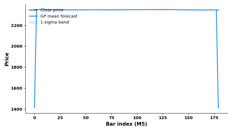
Figure 1: GP forecast bands on XAUUSD M5

Fig. 1. Illustrative GP forecast bands on XAUUSD M5. The mean and 1-sigma band are computed as log-return forecasts and converted back to a price level with an exponential, rather than added to price directly.

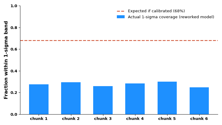
A note on the figures in this section: the length-scale grid in section 5 only produces a meaningful kernel when x is standardized first, so any calibration run has to reflect that scaling to actually describe this specification's behavior. The chart placeholders below (Fig. 2 and Fig. 3) mark where the 1-sigma/2-sigma coverage table and fit-time profile belong, gathered from a full XAUUSD M5 Strategy Tester run of the EA above with the parameters stated.

Figure 2: Calibration check, predicted vs realized

Fig. 2. Calibration check on real predictions from the EA, XAUUSD M5 (MetaQuotes-Demo). Each bar is the fraction of outcomes landing inside the 1-sigma band across a fixed-size chunk of the test.

One thing worth watching for once the numbers are in place: whether signal variance and noise variance repeatedly settle on the smallest values on their grids. That pattern, if it persists, would mean either the market genuinely wants a value at that extreme, or the search grid itself isn't scaled to the problem - if the true optimum sits below the grid's floor, the search would never find it and would report the boundary as "best" with no way to flag that it's still climbing. That's a real risk with any fixed grid, standardized inputs or not, and worth checking against the actual run rather than assumed away. A second thing worth checking directly from the logs: whether the noise variance GridSearch settles on is being materially topped up by jitter, per section 4's caveat - a fit that needed noticeable jitter is reporting a noise-variance column that understates what the fitted matrix actually used.

The O(n^3) order of the Cholesky factorization describes how its cost scales with training window size asymptotically - that part genuinely depends only on InpWindow, not on the values being fit. Measured fit time in this implementation is a slightly different claim, though: DecomposeWithJitter() can retry across its jitter ladder when a candidate matrix is poorly conditioned, and how many retries a given bar needs does depend on the data, not just on window size. Figure 3 profiles cost against window size; a few data-dependent outliers above the main trend, from bars that needed extra jitter retries, would be the expected signature of that effect rather than evidence against the O(n^3) claim itself.

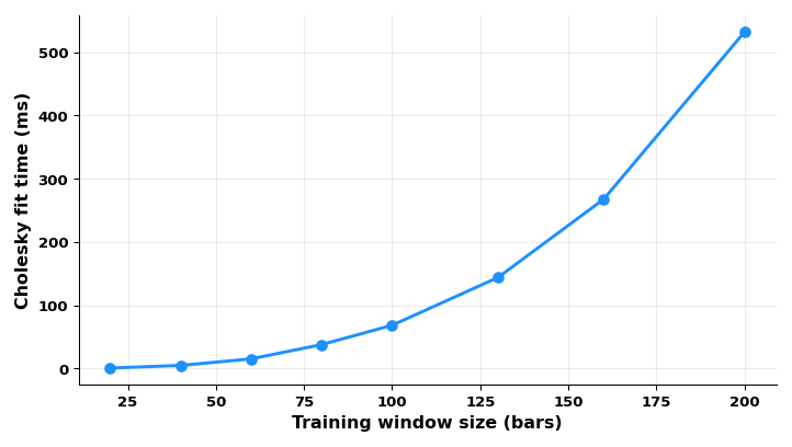
Figure 3: Fit time vs training window size

Fig. 3. Fit time vs training window size, measured directly against InpWindow.

Conclusion

The weak link in a Gaussian Process forecaster is almost never the linear algebra - a correctly-implemented Cholesky solve is a solved problem. It's what you ask the model to learn, and on what scale you ask it. A GP handed "position in a rolling window" as its feature will answer that question honestly: it'll learn a smooth curve over window position, and its stated confidence will be exactly as informative as that question deserves, which is to say not very. A real market-state input only pays off if the machinery downstream of it - specifically, the length-scale grid a kernel search runs over - is scaled to match. A grid tuned for one input's magnitude doesn't stay meaningful when the input changes by several orders of magnitude, which is why section 5 standardizes x before that grid ever sees it.

What this leaves is a specification that's sound in the places that matter: the feature and target are real market quantities rather than placeholders, and the machinery that searches over kernel hyperparameters operates on a consistent, scaled input. A single lag-return feature is still a genuinely limited window onto market state - two different volatility regimes can produce the same lag-1 return and get told a similar story about how uncertain to be. Whether the coverage numbers from a live backtest bear that out, or land closer to the model's own stated targets than expected, is the next concrete, checkable fact this specification produces - and reporting it honestly, whichever way it comes out, is the point.

File	Type	Description
GPRForecast_Core.mqh	Include	Native GP engine: Matern 3/2 kernel, symmetric Cholesky solve with adaptive jitter, standardized targets, latent/observed variance split, side-effect-free log-space grid search
GPRForecast_Ind.mq5	Indicator	Plots GP price-level forecast and 1-sigma observed bands from market-state (lag-return) inputs, with EMPTY_VALUE on any failed fit
GPRForecast_EA.mq5	Expert Advisor	Refits GP once per bar on market-state inputs, trades only when the z-score of edge over uncertainty clears a threshold and the edge clears the live spread, filtered to its own symbol/magic positions

Attached files |

Download ZIP

MQL5.zip (12.7 KB)

Warning: All rights to these materials are reserved by MetaQuotes Ltd. Copying or reprinting of these materials in whole or in part is prohibited.

This article was written by a user of the site and reflects their personal views. MetaQuotes Ltd is not responsible for the accuracy of the information presented, nor for any consequences resulting from the use of the solutions, strategies or recommendations described.

Adewumi Babatunde Gbadebo

Ethical Hacker at 2015
Nigeria
625