

Hidden Semi-Markov Models for Duration-Aware Regime Detection in MQL5
 133
133
 0
0

Introduction
Most regime-detection write-ups use a plain Hidden Markov Model: a handful of states, a transition matrix, and a forward–backward pass to estimate the current state. This assumes a geometric sojourn time: the probability that a regime ends on the next bar is constant, regardless of how long it has lasted. Markets do not behave that way — trends and chop both have momentum in a mean-duration sense.
A Hidden Semi-Markov Model (HSMM) fixes this by pulling duration out of the transition matrix and giving each state its own explicit sojourn-time distribution. The model then carries a live estimate of how much longer the current state is expected to run, which lets an Expert Advisor hold a trend trade through the middle of a move but step aside once that estimate shrinks toward zero.
This follows the same offline-Python/live-native-MQL5 pipeline as earlier regime work in this series, but answers a different question: not just which state this is, but how much of it is probably left.
Scope note: the duration-aware inference engine runs entirely natively in MQL5 — Python is used only offline, to fit parameters via Expectation-Maximization. Everything shown targets XAUUSD M5, though nothing in the math is instrument-specific.
Contents
- Introduction
- Why duration matters: from HMM to HSMM
- Feature engineering: three signals for regime identity
- The duration-aware forward filter
- Reading the manifest: a native JSON bridge between Python and MQL5
- From belief to trade: hysteresis, duration gating, and position sizing
- Visualizing the regime: the indicator's incremental filter
- Edge cases and pitfalls
- Testing in the Strategy Tester
- Conclusion
Why duration matters: from HMM to HSMM
In a standard HMM, the probability of staying in state j for exactly one more bar is the diagonal transition entry, and the probability of staying for exactly k more bars falls out as a geometric distribution:
P(duration = k | state = j) = (A_jj)^(k-1) * (1 - A_jj)
That formula has a mode at k = 1: the single most likely outcome, every bar, is that the regime ends right now — a strange shape for a market regime, since real trends and ranges build up before becoming likely to end. An HSMM replaces this with an explicitly-fitted distribution d_j(k) per state, decoupled from the transition matrix, which keeps only the conditional question of which state comes next once the current one ends.
This project fits d_j(k) as a discretized negative binomial per state, truncated to 60 bars on M5 — a two-parameter family that smooths noisy empirical duration tails while still matching the empirical mean and variance exactly.
Fitted duration distributions per regime state
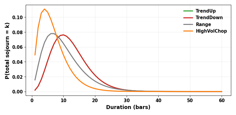
Fig. 1. Discretized negative-binomial duration distributions for the four regime states, as stored in hsmm_manifest.json. TrendUp and TrendDown share a longer, right-shifted duration profile; Range decays fastest; HighVolChop is the shortest-lived state by design, since volatility expansions that do not resolve into a clean trend tend to burn out quickly.
Practically, an HMM encodes remaining time implicitly via a constant transition probability, so it does not depend on regime age. An HSMM's belief about remaining duration is a live, evolving number that shrinks as a regime ages past its distribution's mode and can be read out and acted on directly, bar by bar.
Four states cover what this system needs to distinguish: TrendUp, TrendDown, Range for low-efficiency chop, and HighVolChop for volatility expansions that never resolve into a clean direction — without it, such spikes get misread as an ambiguous blend of the two trend states.
Feature engineering: three signals for regime identity
The emission model scores every closed bar against three features, each computed over a rolling 20-bar window. All three are scale-free ratios rather than raw price or volatility numbers, so the fitted model generalizes across volatility regimes without needing to be refitted every time ATR drifts:
- realized_vol_dev — short-window realized volatility versus what the broker's ATR implies, as a ratio minus one; catches a volatility expansion before ATR catches up.
- efficiency_ratio — Kaufman's net distance/path length ratio: near 1.0 for a clean trend, near 0.0 for chop.
- return_skew — third standardized moment of the return window; separates a slow grind from a panicky one-sided move, giving TrendUp/TrendDown distinct signatures even when volatility and efficiency look similar.
All three formulas live once in CHSMMFilter::ComputeFeatures(), shared verbatim by the EA and the indicator, which rules out training/inference feature skew between them:
//+------------------------------------------------------------------+
//| CHSMMFilter::ComputeFeatures                                     |
//+------------------------------------------------------------------+
bool CHSMMFilter::ComputeFeatures(const double &close[], int shift, double atr_value, double &features_out[])
  {
//--- close[] must be a series-indexed array (ArraySetAsSeries(...,true))
//--- so that close[shift] is the bar we are scoring and close[shift+1]
//--- is one bar older. FEATURE_LOOKBACK+1 closes are required to form
//--- FEATURE_LOOKBACK log-returns, so callers must guarantee that many
//--- bars exist before calling this -- callers should check
//--- Bars(...) >= FEATURE_LOOKBACK+2 before entering their bar loop.
   ArrayResize(features_out, NUM_FEATURES);

   double returns[FEATURE_LOOKBACK];
   for(int i = 0; i < FEATURE_LOOKBACK; i++)
     {
      double c_new = close[shift + i];
      double c_old = close[shift + i + 1];
      if(c_old <= 0.0 || c_new <= 0.0)
         return(false);   // guard: corrupt/zero price would poison MathLog below
      returns[i] = MathLog(c_new / c_old);
     }

//--- feature 0: realized_vol_dev -- how far the SHORT-WINDOW realized
//--- volatility of returns sits from the volatility implied by the
//--- broker's own ATR reading. Zero means "about what ATR would
//--- predict"; a large positive value flags a volatility expansion
//--- that ATR (a slower, smoothed measure) has not yet caught up to
//--- -- exactly the kind of regime break this model is meant to
//--- detect early.
   double mean_r = 0.0;
   for(int i = 0; i < FEATURE_LOOKBACK; i++)
      mean_r += returns[i];
   mean_r /= FEATURE_LOOKBACK;

   double var_r = 0.0;
   for(int i = 0; i < FEATURE_LOOKBACK; i++)
     {
      double d = returns[i] - mean_r;
      var_r += d * d;
     }
   var_r /= FEATURE_LOOKBACK;
   double realized_sigma = MathSqrt(var_r);

   double atr_frac = atr_value / close[shift];
   if(atr_frac < 1e-8)
      atr_frac = 1e-8;   // guard against a zero/near-zero ATR reading on a very quiet symbol
   features_out[0] = (realized_sigma / atr_frac) - 1.0;

//--- feature 1: Kaufman efficiency ratio -- net directional travel
//--- divided by total path length walked to get there, over the same
//--- lookback window. Close to 1.0 means the price moved in a
//--- straight line (a clean trend); close to 0.0 means it wandered
//--- back and forth and ended up near where it started (chop/range).
   double net_change = MathAbs(close[shift] - close[shift + FEATURE_LOOKBACK]);
   double path_sum = 0.0;
   for(int i = 0; i < FEATURE_LOOKBACK; i++)
      path_sum += MathAbs(close[shift + i] - close[shift + i + 1]);
   if(path_sum < 1e-12)
      path_sum = 1e-12;   // guard: a perfectly flat window would otherwise divide by zero
   features_out[1] = net_change / path_sum;

//--- feature 2: return skew -- third standardized moment of the
//--- return window. Distinguishes a slow grinding trend (mildly
//--- skewed) from a panic move (heavily skewed in one direction),
//--- which is useful because two regimes can share similar realized
//--- volatility and efficiency ratio yet have very different skew
//--- signatures.
   double m3 = 0.0;
   for(int i = 0; i < FEATURE_LOOKBACK; i++)
     {
      double d = returns[i] - mean_r;
      m3 += d * d * d;
     }
   m3 /= FEATURE_LOOKBACK;
   double sigma3 = MathPow(realized_sigma, 3.0);
   if(sigma3 < 1e-12)
      sigma3 = 1e-12;   // guard: near-zero variance window would otherwise blow up the ratio
   features_out[2] = m3 / sigma3;

   return(true);
  }
The zero-price guard before MathLog() and the ATR-fraction floor both protect against a real but rare case: a fully illiquid stretch (thin session, feed hiccup) producing a zero-width bar that would otherwise divide by near-zero and inject a meaningless spike into the emission likelihood.
The scatter below shows why these three features separate the four states well enough to fit a Gaussian emission model using a synthetic sequence generated from the manifest's own fitted parameters — a shape sanity-check, not a market-performance claim:
Synthetic feature-space separation across the four regime states
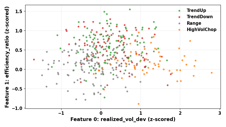
Fig. 2. realized_vol_dev vs. efficiency_ratio for 400 synthetically generated bars, colored by their true generating state. TrendUp and TrendDown cluster at high efficiency; Range sits low on both axes; HighVolChop pulls out along the volatility axis while staying low on efficiency — exactly the separation the emission Gaussians are meant to exploit.
The duration-aware forward filter
This is what makes the model duration-aware in real time — a genuinely different recursion from a textbook HMM forward pass. The belief state is alpha[state][remaining_duration]: each cell holds the probability of being in a state with a given number of bars left before it ends. Every bar, two things can happen to that belief, one deterministic and one probabilistic:
alpha_t(j, d) for d > 0:  mass simply moves to (j, d-1) -- the state continues, deterministically
alpha_{t-1}(j, 0):     the state finishes; mass exits to a NEW state j' ~ A[j][j'],
                          drawing a brand-new duration k ~ duration_pmf[j'], landing on (j', k-1)
The first case is pure bookkeeping — the duration was already drawn on entry, so counting it down costs nothing. The second is where the transition matrix and duration pmf do their work: which state comes next is drawn from the (off-diagonal) transition matrix, and how long it lasts is drawn independently from its duration pmf. This is CHSMMFilter::PredictStep():
//+------------------------------------------------------------------+
//| CHSMMFilter::PredictStep                                         |
//+------------------------------------------------------------------+
void CHSMMFilter::PredictStep(void)
  {
//--- explicit-duration (residual-time) HSMM time update. Each belief
//--- cell alpha[j,d] holds P(state=j, d bars remaining in this state).
//--- Two things can happen to the mass in a cell between bar t-1 and
//--- bar t:
//---   1) d > 0: the state simply continues -- remaining duration
//---      counts down by exactly one, deterministically. No branch,
//---      no probability multiply, because the duration was already
//---      drawn when the state was entered.
//---   2) d == 0: this bar was the LAST bar of the state's sojourn,
//---      so the process transitions OUT to some new state j' (drawn
//---      from the off-diagonal transition matrix) and simultaneously
//---      draws a brand-new total duration k for j' from that state's
//---      duration pmf, landing in cell (j', k-1).
   double pred[NUM_STATES * MAX_DURATION];
   ArrayInitialize(pred, 0.0);

   double finishing[NUM_STATES];
   for(int j = 0; j < NUM_STATES; j++)
      finishing[j] = m_alpha[j * MAX_DURATION + 0];

//--- case 1: deterministic countdown for every cell with d > 0.
   for(int j = 0; j < NUM_STATES; j++)
     {
      for(int d = 1; d < MAX_DURATION; d++)
        {
         double mass = m_alpha[j * MAX_DURATION + d];
         if(mass <= 0.0)
            continue;
         pred[j * MAX_DURATION + (d - 1)] += mass;
        }
     }

//--- case 2: mass finishing state j is redistributed into every
//--- other state j', weighted by the transition probability and by
//--- that state's own duration pmf (which sets its NEW remaining
//--- duration on entry). Truncating k at MAX_DURATION means a tiny
//--- amount of probability mass for exceptionally long regimes is
//--- dropped rather than wrapped or clipped into the last bucket --
//--- an acceptable approximation as long as the duration pmf was fit
//--- so its tail is already small beyond MAX_DURATION bars.
   for(int j = 0; j < NUM_STATES; j++)
     {
      if(finishing[j] <= 0.0)
         continue;
      for(int jp = 0; jp < NUM_STATES; jp++)
        {
         if(jp == j)
            continue;
         double outflow = finishing[j] * m_transition[j * NUM_STATES + jp];
         if(outflow <= 0.0)
            continue;
         for(int k = 1; k <= MAX_DURATION; k++)
           {
            double p_dur = m_duration_pmf[jp * MAX_DURATION + (k - 1)];
            if(p_dur <= 0.0)
               continue;
            pred[jp * MAX_DURATION + (k - 1)] += outflow * p_dur;
           }
        }
     }

   ArrayCopy(m_alpha, pred);
  }
Truncating at MAX_DURATION drops a small amount of mass for very long regimes instead of folding it into the last bucket. This is acceptable if the duration-PMF tail is already small by 60 bars, which training enforces via negative-binomial smoothing.
Once the belief is rolled forward, the closed bar's features are folded in as a Bayesian likelihood update — every cell belonging to state j is multiplied by that state's Gaussian emission likelihood, since duration does not affect the emission by construction:
//+------------------------------------------------------------------+
//| CHSMMFilter::GaussianLogLik                                      |
//+------------------------------------------------------------------+
double CHSMMFilter::GaussianLogLik(int state, const double &norm_features[])
  {
//--- diagonal-covariance multivariate Gaussian log-density, summed
//--- feature-by-feature. Working in log space (rather than
//--- multiplying raw densities together) avoids underflow to exactly
//--- zero when several features are simultaneously several standard
//--- deviations from a state's mean -- a real risk once NUM_FEATURES
//--- and the number of states both grow.
   double log_lik = 0.0;
   for(int f = 0; f < NUM_FEATURES; f++)
     {
      double var = m_emission_var[state * NUM_FEATURES + f];
      if(var < 1e-8)
         var = 1e-8;    // guard: a state that saw almost no feature variance during training
      double mean = m_emission_mean[state * NUM_FEATURES + f];
      double diff = norm_features[f] - mean;
      log_lik += -0.5 * MathLog(2.0 * M_PI * var) - 0.5 * (diff * diff) / var;
     }
   return(log_lik);
  }

//+------------------------------------------------------------------+
//| CHSMMFilter::UpdateStep                                          |
//+------------------------------------------------------------------+
void CHSMMFilter::UpdateStep(const double &raw_features[])
  {
//--- Bayesian measurement update: multiply every (state,duration)
//--- cell by that state's emission likelihood for the bar just
//--- closed, then renormalize. Duration does not affect the
//--- emission -- by construction the observation model only reads
//--- the discrete regime label, not how long it has been active --
//--- so every cell belonging to state j gets the SAME multiplier.
   double norm_features[];
   NormalizeFeatures(raw_features, norm_features);

   double log_lik[NUM_STATES];
   double max_log_lik = -DBL_MAX;
   for(int j = 0; j < NUM_STATES; j++)
     {
      log_lik[j] = GaussianLogLik(j, norm_features);
      if(log_lik[j] > max_log_lik)
         max_log_lik = log_lik[j];
     }

//--- numerically stable exponentiation: subtract the max log-lik
//--- before calling MathExp() so the largest term becomes exp(0)=1
//--- and every other term is a well-behaved value in (0,1], instead
//--- of risking exp() underflow/overflow on raw log-likelihoods that
//--- can run to several hundred in magnitude.
   double lik[NUM_STATES];
   for(int j = 0; j < NUM_STATES; j++)
      lik[j] = MathExp(log_lik[j] - max_log_lik);

   double total = 0.0;
   for(int j = 0; j < NUM_STATES; j++)
     {
      for(int d = 0; d < MAX_DURATION; d++)
        {
         m_alpha[j * MAX_DURATION + d] *= lik[j];
         total += m_alpha[j * MAX_DURATION + d];
        }
     }

//--- renormalize so the belief stays a proper probability
//--- distribution. If total collapses to (near) zero -- e.g. after
//--- many bars of extremely unlikely observations under every state
//--- -- fall back to a fresh uniform prior rather than dividing by
//--- (near) zero and injecting NaNs into the belief state.
   if(total < 1e-300)
     {
      ResetBelief();
      return;
     }
   for(int i = 0; i < NUM_STATES * MAX_DURATION; i++)
      m_alpha[i] /= total;
  }
The max-subtraction before MathExp() is not decorative: raw log-likelihoods can run to hundreds in magnitude, and exponentiating directly risks overflow or silent underflow to zero — which would make the filter act artificially certain. Subtracting the max first keeps every term in a well-behaved [0,1] range.
To make a decision, marginalize over duration to estimate the state, then compute the expected remaining duration as a duration-weighted average. ManageTrades() uses this value; a plain HMM has no direct analogue:
//+------------------------------------------------------------------+
//| CHSMMFilter::StepFilter                                          |
//+------------------------------------------------------------------+
void CHSMMFilter::StepFilter(const double &raw_features[])
  {
//--- convenience wrapper: advance the belief by exactly one closed
//--- bar. Predict must run BEFORE Update -- Predict propagates last
//--- bar's posterior forward through the countdown/transition
//--- dynamics to form this bar's prior, and only then does Update
//--- fold in this bar's actual observation. Calling these in the
//--- opposite order would condition on an observation before the
//--- state had even been allowed to evolve, which is not the filter
//--- this class is documented to implement.
   PredictStep();
   UpdateStep(raw_features);
  }

//+------------------------------------------------------------------+
//| CHSMMFilter::GetFilteredState                                    |
//+------------------------------------------------------------------+
int CHSMMFilter::GetFilteredState(double &confidence)
  {
//--- marginalizes the belief over duration to get P(state=j) for
//--- each state, then returns the argmax and its probability mass as
//--- a confidence score the caller can threshold against before
//--- acting on a regime call.
   double state_prob[NUM_STATES];
   for(int j = 0; j < NUM_STATES; j++)
     {
      double s = 0.0;
      for(int d = 0; d < MAX_DURATION; d++)
         s += m_alpha[j * MAX_DURATION + d];
      state_prob[j] = s;
     }
   int best = 0;
   for(int j = 1; j < NUM_STATES; j++)
      if(state_prob[j] > state_prob[best])
         best = j;
   confidence = state_prob[best];
   return(best);
  }

//+------------------------------------------------------------------+
//| CHSMMFilter::GetExpectedRemainingDuration                        |
//+------------------------------------------------------------------+
double CHSMMFilter::GetExpectedRemainingDuration(int state)
  {
//--- E[remaining bars | state=j] = sum_d d * alpha[j,d] / sum_d alpha[j,d].
//--- This is the number that makes the model "duration-aware" in a way
//--- a plain HMM's transition-matrix diagonal never gives you directly:
//--- a caller can gate entries on the regime STILL having runway left,
//--- not just on which regime is currently most likely.
   double num = 0.0, den = 0.0;
   for(int d = 0; d < MAX_DURATION; d++)
     {
      double mass = m_alpha[state * MAX_DURATION + d];
      num += d * mass;
      den += mass;
     }
   if(den < 1e-12)
      return(0.0);
   return(num / den);
  }
E[remaining bars | state=j] = sum_d( d * alpha[j,d] ) / sum_d( alpha[j,d] )
When run over a synthetic 400-bar sequence from the manifest's own parameters, the filter recovers the true generating regime on roughly three of every four bars — a useful sanity check before pointing the recursion at real data:
Filtered regime posterior over a synthetic 400-bar sequence
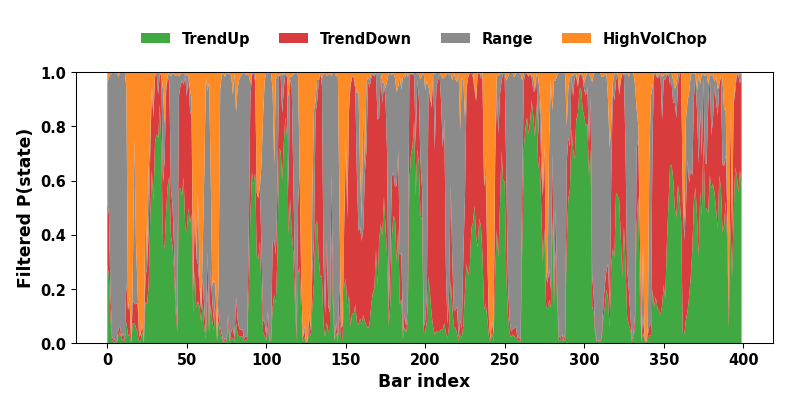
Fig. 3. Stacked filtered posterior P(state) over 400 synthetic bars. Each band's height is that state's current belief probability; the model tracks the underlying (known, synthetically generated) regime switches with a short lag, which is the expected behavior of any causal filter — it only ever conditions on the past.
Reading the manifest: a native JSON bridge between Python and MQL5
The offline EM script exports all fitted parameters to hsmm_manifest.json (emissions, transition matrix, duration PMFs, normalization stats). MQL5 has no built-in JSON parser to load it. Rather than pull in a full JSON grammar for a manifest with a small, fixed key set, CJSONArrayUtils implements just two operations: pulling a named field's raw value out of the document, and flattening a numeric array of any nesting depth into a row-major buffer. Both lean on the same trick — tracking bracket depth ('[' or '{') as the scan proceeds and only treating a comma or closing bracket as a boundary at depth zero — which is what lets SplitTopLevel() recurse safely on nested arrays:
void CJSONArrayUtils::SplitTopLevel(string s, string &parts_out[])
  {
//--- splits a comma-separated JSON list at commas that sit at
//--- bracket-depth zero only. A manifest field such as
//--- "[[1,2],[3,4]]" must NOT be split at the commas that separate
//--- 1 from 2, only at the comma that separates the two inner
//--- arrays -- so we track '[' / '{' depth as we scan and only
//--- treat a comma as a delimiter when depth == 0.
   ArrayResize(parts_out, 0);
   int depth = 0;
   int start = 0;
   int len = StringLen(s);
   for(int i = 0; i < len; i++)
     {
      ushort c = StringGetCharacter(s, i);
      if(c == '[' || c == '{')
         depth++;
      else if(c == ']' || c == '}')
         depth--;
      else if(c == ',' && depth == 0)
        {
         string token = StringSubstr(s, start, i - start);
         StringTrimLeft(token);
         StringTrimRight(token);
         int n = ArraySize(parts_out);
         ArrayResize(parts_out, n + 1);
         parts_out[n] = token;
         start = i + 1;
        }
     }
//--- flush the final token -- there is no trailing comma after the
//--- last element, so the loop above never emits it on its own.
   string last_token = StringSubstr(s, start, len - start);
   StringTrimLeft(last_token);
   StringTrimRight(last_token);
   if(StringLen(last_token) > 0)
     {
      int n2 = ArraySize(parts_out);
      ArrayResize(parts_out, n2 + 1);
      parts_out[n2] = last_token;
     }
  }
ExtractValueRaw() applies the same idea to capture a bracketed field value whole, instead of cutting it off at the first internal comma the way a plain StringFind()-to-next-comma approach would:
string CJSONArrayUtils::ExtractValueRaw(string json, string key)
  {
//--- returns the raw (still JSON-encoded) value text that follows
//--- "\"key\":" inside json, respecting bracket depth so a value that
//--- is itself an object/array is captured whole rather than cut off
//--- at its first internal comma. This is a targeted extractor (not
//--- a general parser) because the manifest has a small, fixed key
//--- set -- a full recursive-descent grammar would be more code for
//--- no practical benefit here.
   string needle = "\"" + key + "\":";
   int pos = StringFind(json, needle);
   if(pos < 0)
      return("");
   int cursor = pos + StringLen(needle);
   int len = StringLen(json);
//--- skip whitespace between the colon and the value proper.
   while(cursor < len && StringGetCharacter(json, cursor) == ' ')
      cursor++;
   ushort first = StringGetCharacter(json, cursor);
   int start = cursor;
   if(first == '[' || first == '{')
     {
      //--- bracketed value: walk forward counting depth until the
      //--- matching close bracket is found.
      ushort open_ch  = first;
      ushort close_ch = (first == '[') ? ']' : '}';
      int depth = 0;
      for(int i = cursor; i < len; i++)
        {
         ushort c = StringGetCharacter(json, i);
         if(c == open_ch)
            depth++;
         else if(c == close_ch)
           {
            depth--;
            if(depth == 0)
               return(StringSubstr(json, start, i - start + 1));
           }
        }
      return(StringSubstr(json, start, len - start));
     }
   else if(first == '"')
     {
      //--- quoted string value: find the closing quote.
      int i = cursor + 1;
      while(i < len && StringGetCharacter(json, i) != '"')
         i++;
      return(StringSubstr(json, start, i - start + 1));
     }
   else
     {
      //--- bare number/literal: ends at the next comma or closing
      //--- brace at the current (top) level.
      int i = cursor;
      while(i < len)
        {
         ushort c = StringGetCharacter(json, i);
         if(c == ',' || c == '}' || c == '\n' || c == '\r')
            break;
         i++;
        }
      return(StringSubstr(json, start, i - start));
     }
  }
With those two primitives in place, LoadManifest() reads the whole file, pulls out every field by name, and copies each parsed array into the class's fixed-size member arrays index-for-index:
bool CHSMMFilter::LoadManifest(string filename)
  {
   string json;
   if(!ReadWholeFile(filename, json))
      return(false);

//--- scalar contract fields -- read first so ValidateContract() can
//--- reject a mismatched manifest before we waste time parsing the
//--- (potentially large) numeric arrays below.
   m_manifest_num_states   = (int)StringToInteger(CJSONArrayUtils::ExtractValueRaw(json, "num_states"));
   m_manifest_max_duration = (int)StringToInteger(CJSONArrayUtils::ExtractValueRaw(json, "max_duration"));

//--- feature_names is an array; its element COUNT (not its content)
//--- is what the three-way contract actually checks against
//--- NUM_FEATURES -- there is no separate scalar "feature count"
//--- field in the manifest, since that would just be a second source
//--- of truth that could itself drift out of sync with the array.
   string feat_names_raw = CJSONArrayUtils::ExtractValueRaw(json, "feature_names");
   string feat_name_tokens[];
   CJSONArrayUtils::SplitTopLevel(CJSONArrayUtils::StripBrackets(feat_names_raw), feat_name_tokens);
   m_manifest_num_features = ArraySize(feat_name_tokens);

   if(!ValidateContract())
      return(false);

//--- numeric parameter blocks -- each parsed into a flat double
//--- array via CJSONArrayUtils::ParseDoubleArray, then copied into
//--- the fixed-size member arrays index-for-index (row-major, so
//--- emission_mean[state][feature] lives at state*NUM_FEATURES+feature).
   double tmp[];

   CJSONArrayUtils::ParseDoubleArray(CJSONArrayUtils::ExtractValueRaw(json, "emission_mean"), tmp);
   for(int i = 0; i < ArraySize(tmp) && i < NUM_STATES * NUM_FEATURES; i++)
      m_emission_mean[i] = tmp[i];

   CJSONArrayUtils::ParseDoubleArray(CJSONArrayUtils::ExtractValueRaw(json, "emission_var"), tmp);
   for(int i = 0; i < ArraySize(tmp) && i < NUM_STATES * NUM_FEATURES; i++)
      m_emission_var[i] = tmp[i];

   CJSONArrayUtils::ParseDoubleArray(CJSONArrayUtils::ExtractValueRaw(json, "transition_matrix"), tmp);
   for(int i = 0; i < ArraySize(tmp) && i < NUM_STATES * NUM_STATES; i++)
      m_transition[i] = tmp[i];

   CJSONArrayUtils::ParseDoubleArray(CJSONArrayUtils::ExtractValueRaw(json, "duration_pmf"), tmp);
   for(int i = 0; i < ArraySize(tmp) && i < NUM_STATES * MAX_DURATION; i++)
      m_duration_pmf[i] = tmp[i];

   CJSONArrayUtils::ParseDoubleArray(CJSONArrayUtils::ExtractValueRaw(json, "feature_norm_mean"), tmp);
   for(int i = 0; i < ArraySize(tmp) && i < NUM_FEATURES; i++)
      m_feat_norm_mean[i] = tmp[i];

   CJSONArrayUtils::ParseDoubleArray(CJSONArrayUtils::ExtractValueRaw(json, "feature_norm_std"), tmp);
   for(int i = 0; i < ArraySize(tmp) && i < NUM_FEATURES; i++)
      m_feat_norm_std[i] = tmp[i];

//--- state_names is a string array, not numeric, so it gets its own
//--- lightweight split-and-strip-quotes pass rather than reusing
//--- ParseDoubleArray.
   string names_raw = CJSONArrayUtils::ExtractValueRaw(json, "state_names");
   string name_tokens[];
   CJSONArrayUtils::SplitTopLevel(CJSONArrayUtils::StripBrackets(names_raw), name_tokens);
   for(int i = 0; i < ArraySize(name_tokens) && i < NUM_STATES; i++)
     {
      string t = name_tokens[i];
      StringTrimLeft(t);
      StringTrimRight(t);
      StringReplace(t, "\"", "");
      m_state_names[i] = t;
     }

   m_loaded = true;
   ResetBelief();
   Print("CHSMMFilter: manifest loaded OK from ", filename);
   return(true);
  }
The scalar contract fields — num_states, max_duration, and the feature_names count — are parsed and validated before any of the large numeric arrays, via ValidateContract():
bool CHSMMFilter::ValidateContract(void)
  {
//--- the three-way contract: compile-time constants, manifest
//--- fields, and (implicitly, via array sizes above) the actual
//--- parsed array lengths must all agree. We fail loudly here rather
//--- than silently truncating or padding a mismatched array, because
//--- a silent truncation would let the EA run with a corrupted model
//--- and produce plausible-looking but meaningless regime calls.
   bool ok = true;
   if(m_manifest_num_states != NUM_STATES)
     {
      Print("CHSMMFilter: CONTRACT MISMATCH -- manifest num_states=", m_manifest_num_states,
            " but compiled NUM_STATES=", NUM_STATES);
      ok = false;
     }
   if(m_manifest_num_features != NUM_FEATURES)
     {
      Print("CHSMMFilter: CONTRACT MISMATCH -- manifest feature_names count=", m_manifest_num_features,
            " but compiled NUM_FEATURES=", NUM_FEATURES);
      ok = false;
     }
   if(m_manifest_max_duration != MAX_DURATION)
     {
      Print("CHSMMFilter: CONTRACT MISMATCH -- manifest max_duration=", m_manifest_max_duration,
            " but compiled MAX_DURATION=", MAX_DURATION);
      ok = false;
     }
   return(ok);
  }
A mismatched manifest — say, trained with five states after NUM_STATES changed without recompiling — is not silently truncated or zero-padded: OnInit() returns INIT_FAILED and the EA refuses to start, rather than trading on a belief state built from a corrupted model.
The manifest comes from train_hsmm.py, run offline against an MetaTader 5-exported OHLC history. Two quirks are handled at CSV import: MetaTrader 5's FILE_CSV writer emits UTF-16, not UTF-8, and the delimiter follows the terminal's regional settings rather than a fixed comma:
def load_mt5_csv(path):
    """
    Loads an OHLC history CSV as exported from the MT5 terminal.

    Two MT5-specific quirks are handled here rather than left for pandas'
    defaults to mangle silently:
      - MT5's FILE_CSV writer emits UTF-16, not UTF-8, so a plain
        pd.read_csv() call would either raise or -- worse -- succeed
        while reading garbage.
      - The column delimiter follows the terminal's Windows regional
        setting (comma OR semicolon depending on locale), so we let
        pandas' python engine sniff it via sep=None rather than hard-
        coding one and having the import silently misparse on a
        different machine.
    """
    df = pd.read_csv(path, sep=None, engine="python", encoding="utf-16")
    # a UTF-16 BOM sometimes survives as a literal character glued onto
    # the first column name (e.g. "\ufeffTime") -- strip it so column
    # lookups by name don't mysteriously fail.
    df.columns = [c.replace("\ufeff", "") for c in df.columns]
    df = df.rename(columns={c: c.strip().lower() for c in df.columns})
    df = df.sort_values("time" if "time" in df.columns else df.columns[0])
    df = df.reset_index(drop=True)
compute_features() is a term-for-term Python port of CHSMMFilter::ComputeFeatures() from Section 4, vectorized with numpy but not restructured, since the two must agree bar-for-bar on what a feature value means:
def compute_features(close, atr):
    """
    Builds the same three features CHSMMFilter::ComputeFeatures()
    computes on the MQL5 side, over a rolling FEATURE_LOOKBACK window.
    Vectorized with numpy for training-time speed across a full history,
    but the underlying formulas are deliberately kept identical,
    term-for-term, to the MQL5 implementation.

    Returns an (N - FEATURE_LOOKBACK, NUM_FEATURES) array; row i
    corresponds to bar index i + FEATURE_LOOKBACK in the original series.
    """
    close = np.asarray(close, dtype=np.float64)
    atr = np.asarray(atr, dtype=np.float64)
    n = len(close)
    log_ret = np.diff(np.log(close))  # log_ret[t] = ln(close[t+1]/close[t])

    n_rows = n - FEATURE_LOOKBACK
    feats = np.zeros((n_rows, NUM_FEATURES), dtype=np.float64)

    for row, t in enumerate(range(FEATURE_LOOKBACK, n)):
        # window of returns ending at bar t: the FEATURE_LOOKBACK returns
        # immediately preceding it, matching CHSMMFilter's
Fitting proceeds as an EM loop, a Baum–Welch analogue extended with an explicit duration dimension. The E-step runs a full forward-and-backward pass over the whole sequence — unlike the online MQL5 filter, which only conditions on the past — producing smoothed posteriors over both state and remaining duration:
def forward_backward_hsmm(feats, trans, dur_pmf, em_mean, em_var):
    """
    Full (non-truncated-for-real-time) explicit-duration forward-backward
    pass over the WHOLE training sequence, used only inside the EM loop.
    This differs from CHSMMFilter's online PredictStep()/UpdateStep() in
    one important way: it also runs a BACKWARD pass, giving smoothed
    (not just filtered) state/duration posteriors -- appropriate for
    offline parameter estimation, where the whole sequence is already
    available, but not something the live EA can do (it only ever sees
    the past).

    Returns:
      gamma:      (T, NUM_STATES)               smoothed P(state=j | all data)
      xi_finish:  (T, NUM_STATES, NUM_STATES)    smoothed P(state j finishes and
                                                  transitions to j' at time t)
      dur_gamma:  (T, NUM_STATES, MAX_DURATION)  smoothed P(state=j, remaining=d)
      total_loglik: float                        true data log-likelihood under the
                                                  CURRENT parameters, log P(O_1:T),
                                                  accumulated from the forward pass's
                                                  own normalizing constants -- this is
                                                  what should actually be tracked for
                                                  EM convergence, not a property of
                                                  gamma (which sums to 1 by
                                                  construction at every t and so
                                                  carries no information about fit
                                                  quality at all).
    """
    T = feats.shape[0]

    # emission log-likelihoods, precomputed once per state for the whole
    # sequence -- this is the single most expensive step per EM
    # iteration, so it is deliberately hoisted out of the T-length loops
    # below rather than recomputed per time step.
    loglik = np.zeros((T, NUM_STATES))
    for j in range(NUM_STATES):
        loglik[:, j] = gaussian_logpdf_diag(feats, em_mean[j], em_var[j])
    lik = np.exp(loglik - loglik.max(axis=1, keepdims=True))

    # forward pass -- same recursion as CHSMMFilter::PredictStep() /
    # UpdateStep(), just kept in an explicit (T, NUM_STATES, MAX_DURATION)
    # array instead of updated in place, because the backward pass below
    # needs every time step's alpha, not just the latest one.
    #
    # This is also a SCALED forward pass in the classic HMM sense: each
    # step's normalizing constant (the total probability mass before
    # dividing it back down to 1) is itself meaningful -- summed in log
    # space across all T steps, it IS the true log-likelihood of the
    # whole observed sequence under the current parameters. Discarding
    # these constants (as an earlier version of this function did) throws
    # away the one number EM convergence should actually be checked
    # against.
    alpha = np.zeros((T, NUM_STATES, MAX_DURATION))
    alpha[0] = 1.0 / (NUM_STATES * MAX_DURATION)
    alpha[0] *= lik[0][:, None]
    c0 = alpha[0].sum()
    alpha[0] /= max(c0, 1e-300)
    # lik[t] = exp(loglik[t] - loglik[t].max()) for numerical stability,
    # which scales every state's likelihood at time t down by a uniform
    # factor of exp(-loglik[t].max()). The true (unscaled) normalizing
    # constant is therefore this step's computed total multiplied back
    # up by exp(+loglik[t].max()) -- i.e. ADD the max back on in log
    # space, not subtract it.
    total_loglik = np.log(max(c0, 1e-300)) + loglik[0].max()

    for t in range(1, T):
        pred = np.zeros((NUM_STATES, MAX_DURATION))
        finishing = alpha[t - 1, :, 0]
        pred[:, :-1] += alpha[t - 1, :, 1:]
        for j in range(NUM_STATES):
            if finishing[j] <= 0:
                continue
            for jp in range(NUM_STATES):
                if jp == j:
                    continue
                outflow = finishing[j] * trans[j, jp]
                if outflow <= 0:
                    continue
                pred[jp, :] += outflow * dur_pmf[jp, :]
        pred *= lik[t][:, None]
        total = pred.sum()
        alpha[t] = pred / total if total > 1e-300 else 1.0 / (NUM_STATES * MAX_DURATION)
        total_loglik += np.log(max(total, 1e-300)) + loglik[t].max()

    # backward pass -- mirror recursion run from T-1 down to 0.
    beta = np.zeros((T, NUM_STATES, MAX_DURATION))
    beta[T - 1] = 1.0
    for t in range(T - 2, -1, -1):
        nxt = beta[t + 1] * lik[t + 1][:, None]
        b = np.zeros((NUM_STATES, MAX_DURATION))
        # continuing (d>0 at t maps to d-1 at t+1)
        b[:, 1:] += nxt[:, :-1]
        # finishing (d==0 at t): probability mass flows out via
        # transition+duration draw, symmetric to the forward pass.
        for j in range(NUM_STATES):
            acc = 0.0
            for jp in range(NUM_STATES):
                if jp == j:
                    continue
                acc += trans[j, jp] * np.sum(dur_pmf[jp, :] * nxt[jp, :])
            b[j, 0] += acc
        s = b.sum()
        beta[t] = b / s if s > 1e-300 else 1.0

    post = alpha * beta
    post /= post.sum(axis=(1, 2), keepdims=True)
    gamma = post.sum(axis=2)                       # (T, NUM_STATES)
    dur_gamma = post                                # (T, NUM_STATES, MAX_DURATION)

    # xi_finish[t, j, jp]: smoothed probability that state j finished
    # (d==0) at time t and the NEXT state is jp -- this is what drives
    # the transition-matrix M-step below.
    xi_finish = np.zeros((T - 1, NUM_STATES, NUM_STATES))
    for t in range(T - 1):
        finishing = alpha[t, :, 0]
        for j in range(NUM_STATES):
            if finishing[j] <= 0:
                continue
            for jp in range(NUM_STATES):
                if jp == j:
                    continue
                mass = finishing[j] * trans[j, jp] * np.sum(dur_pmf[jp, :] * beta[t + 1, jp, :] * lik[t + 1, jp])
                xi_finish[t, j, jp] = mass
        s = xi_finish[t].sum()
        if s > 1e-300:
            xi_finish[t] /= s

    return gamma, xi_finish, dur_gamma, total_loglik
The forward pass mirrors CHSMMFilter::PredictStep()/UpdateStep() from Section 5, run once per EM iteration over the whole training set rather than once per live bar. total_loglik accumulates each step's true log-likelihood in log space — the quantity EM convergence is actually checked against. The backward pass mirrors this in reverse, and together they produce the smoothed posteriors (gamma, dur_gamma, xi_finish) the M-step below is built from.
The M-step's duration re-estimation departs from fitting the raw histogram directly: with limited data, the tail bins (durations near 60 bars) get noisy soft-counts and can leave zero-probability gaps that would wrongly veto a real long regime live. Fitting a two-parameter negative binomial via method-of-moments regularizes the curve into a smooth shape while still matching the empirical mean and variance exactly:
def fit_negative_binomial_moments(weighted_durations, weights):
    """
    Fits a negative-binomial duration distribution to a WEIGHTED sample
    of durations via method-of-moments, then discretizes its pmf over
    1..MAX_DURATION.

    Why parametric smoothing instead of just normalizing the raw
    weighted histogram: with limited training data, the tail bins (long
    durations) get very few effective soft-counts, so a raw histogram's
    tail is noisy and can even contain isolated zero-probability gaps
    that would incorrectly veto a real long-running regime live. Fitting
    a two-parameter negative binomial regularizes the whole curve to a
    smooth, monotonically-plausible shape while still matching the
    empirical mean and variance exactly.
    """
    mean = np.average(weighted_durations, weights=weights)
    var = np.average((weighted_durations - mean) ** 2, weights=weights)
    var = max(var, mean + 1e-6)  # negative binomial requires var > mean
    p = mean / var
    r = mean * p / (1 - p)
    r = max(r, 1e-3)

    k = np.arange(1, MAX_DURATION + 1)
    # shift the standard NB(support 0,1,2,...) so k=1 is the minimum
    # possible sojourn length of one bar.
    pmf = stats.nbinom.pmf(k - 1, r, p)
    pmf = pmf / pmf.sum()
    return pmf
All three M-steps above — emissions, transitions, durations — run inside run_em(), which also owns the k-means warm start and the convergence loop. One detail worth pointing out: the state labels k-means produces are arbitrary and can come out in a different order on every run, which would make STATE_NAMES[0] mean a different thing each time the script is rerun. The order/remap lines immediately after k-means fix that by sorting the initial centroids on a consistent axis (high realized-vol-deviation and low efficiency first) before anything downstream ever sees a state index:
def run_em(feats):
    T = feats.shape[0]

    # --- initialization via k-means (warm start) -------------------
    from scipy.cluster.vq import kmeans2
    centroids, labels = kmeans2(feats, NUM_STATES, minit="++", seed=42)
    # order states by their realized_vol_dev / efficiency_ratio profile
    # so state indices line up with STATE_NAMES in a stable, inspectable
    # way run-to-run rather than an arbitrary k-means label order.
    order = np.lexsort((centroids[:, 1], -centroids[:, 0]))
    remap = {old: new for new, old in enumerate(order)}
    labels = np.array([remap[l] for l in labels])
    centroids = centroids[order]

    em_mean = centroids.copy()
    em_var = np.ones((NUM_STATES, NUM_FEATURES)) * 0.5

    trans = np.full((NUM_STATES, NUM_STATES), 1.0 / (NUM_STATES - 1))
    np.fill_diagonal(trans, 0.0)

    dur_pmf = np.zeros((NUM_STATES, MAX_DURATION))
    for j in range(NUM_STATES):
        dur_pmf[j] = fit_negative_binomial_moments(np.arange(1, MAX_DURATION + 1),
                                                     np.ones(MAX_DURATION))

    prev_loglik = -np.inf
    for it in range(EM_ITERATIONS):
        gamma, xi_finish, dur_gamma, cur_loglik = forward_backward_hsmm(feats, trans, dur_pmf, em_mean, em_var)

        # --- M-step: emissions ---------------------------------
        for j in range(NUM_STATES):
            w = gamma[:, j]
            wsum = w.sum()
            if wsum < 1e-8:
                continue
            em_mean[j] = np.average(feats, axis=0, weights=w)
            diff = feats - em_mean[j]
            em_var[j] = np.average(diff ** 2, axis=0, weights=w)

        # --- M-step: transition matrix (off-diagonal only) -----
        trans_counts = xi_finish.sum(axis=0)
        for j in range(NUM_STATES):
            row_sum = trans_counts[j].sum()
            if row_sum > 1e-8:
                trans[j] = trans_counts[j] / row_sum
            trans[j, j] = 0.0

        # --- M-step: duration distributions ---------------------
        for j in range(NUM_STATES):
            d_values = np.arange(1, MAX_DURATION + 1)
            weights = dur_gamma[:, j, :].sum(axis=0)  # soft count per duration bucket, this state
            if weights.sum() < 1e-6:
                continue
            dur_pmf[j] = fit_negative_binomial_moments(d_values, weights)

        # --- convergence check -----------------------------------
        # cur_loglik is the TRUE data log-likelihood under the
        # parameters used to run the E-step above (i.e. the parameters
        # as of the END of the previous iteration's M-step) -- this is
        # exactly the quantity EM's monotonic-improvement guarantee
        # applies to, and it is expected to increase (or hold flat)
        # every iteration until convergence.
        print(f"EM iteration {it+1:2d}: loglik={cur_loglik:.1f}")
        if abs(cur_loglik - prev_loglik) < EM_TOLERANCE * max(1.0, abs(prev_loglik)):
            print("EM converged.")
            break
        prev_loglik = cur_loglik

    return em_mean, em_var, trans, dur_pmf
Every fitted array — emission means and variances, the transition matrix, four duration pmfs, feature normalization stats, plus bookkeeping metadata like the training-bar count and date — gets serialized into the JSON manifest in exactly the schema CHSMMFilter::LoadManifest() expects, closing the loop between this offline script and the live MQL5 side covered above.
From belief to trade: hysteresis, duration gating, and position sizing
HSMM_RegimeEA.mq5 loads the manifest once, in OnInit(), and refuses to start if either the manifest fails to load or its ATR handle cannot be created — both are hard prerequisites, so failing fast beats limping along with half-initialized state:
//+------------------------------------------------------------------+
//| OnInit                                                           |
//+------------------------------------------------------------------+
int OnInit()
  {
//--- cold-start bootstrap: before any bars have been processed there
//--- is no meaningful "confirmed" regime yet, so we start pending on
//--- Range (the most conservative label -- it authorizes no trend
//--- trades) rather than defaulting to state 0, which would otherwise
//--- look like an immediate (and unearned) TrendUp confirmation.
   g_confirmed_state = REGIME_RANGE;
   g_pending_state   = REGIME_RANGE;
   g_pending_count   = 0;
   g_last_bar_time   = 0;

   if(!g_filter.LoadManifest(InpManifestFilename))
     {
      Print("HSMM_RegimeEA: manifest load/contract check failed, refusing to start.");
      return(INIT_FAILED);
     }

   g_atr_handle = iATR(_Symbol, _Period, InpATRPeriod);
   if(g_atr_handle == INVALID_HANDLE)
     {
      Print("HSMM_RegimeEA: failed to create ATR handle, err=", GetLastError());
      return(INIT_FAILED);
     }

   g_trade.SetExpertMagicNumber(InpMagic);

   if(!OpenLogFile())
      return(INIT_FAILED);

   Print("HSMM_RegimeEA: initialized OK on ", _Symbol, " ", EnumToString(_Period));
   return(INIT_SUCCEEDED);
  }
The confirmed regime is seeded to REGIME_RANGE rather than state 0, since defaulting to state 0 would look like an already-confirmed TrendUp call rather than an arbitrary array index — Range is the most conservative label, authorizing no trend trades on its own.
The raw filtered state can flicker bar-to-bar whenever two states carry near-equal posterior mass. UpdateConfirmedState() gates a change behind two conditions: the new state must clear a minimum confidence threshold, and persist for a run of consecutive bars, before it replaces the value ManageTrades() acts on:
//+------------------------------------------------------------------+
//| UpdateConfirmedState                                             |
//+------------------------------------------------------------------+
void UpdateConfirmedState(int raw_state, double confidence)
  {
//--- hysteresis gate: the raw filtered state can flicker bar-to-bar
//--- whenever two states have close-to-equal posterior mass. Acting
//--- on every flicker would open and close trades on noise, so a new
//--- state must (a) clear a minimum confidence bar AND (b) be seen
//--- for InpConfirmBars CONSECUTIVE bars before it replaces
//--- g_confirmed_state, which is the only variable ManageTrades()
//--- ever reads.
   if(confidence < InpConfirmThreshold)
     {
      //--- low-confidence bar: does not break an existing pending
      //--- streak (a single ambiguous bar shouldn't reset progress),
      //--- but it also does not advance it.
      return;
     }

   if(raw_state == g_confirmed_state)
     {
      g_pending_state = g_confirmed_state;
      g_pending_count = 0;
      return;
     }

   if(raw_state == g_pending_state)
      g_pending_count++;
   else
     {
      g_pending_state = raw_state;
      g_pending_count = 1;
     }

   if(g_pending_count >= InpConfirmBars)
     {
      Print("HSMM_RegimeEA: regime confirmed change ", g_filter.StateName(g_confirmed_state),
            " -> ", g_filter.StateName(g_pending_state));
      g_confirmed_state = g_pending_state;
      g_pending_count = 0;
     }
  }
Position sizing goes through OrderCalcProfit() rather than SYMBOL_TRADE_TICK_VALUE, deliberately — tick value has produced misleading sizing on metals and index CFDs elsewhere in this series. Asking the terminal directly what one lot would gain or lose over the exact stop distance sidesteps that, since it uses the same pricing engine that fills the real order:
//+------------------------------------------------------------------+
//| CalculateLotSize                                                 |
//+------------------------------------------------------------------+
double CalculateLotSize(ENUM_ORDER_TYPE order_type, double entry_price, double sl_price)
  {
//--- risk-normalized sizing: convert the requested percent-of-equity
//--- risk into a lot size that actually loses that much money if
//--- price reaches sl_price. SYMBOL_TRADE_TICK_VALUE is documented
//--- to return misleading figures on some brokers/instruments (seen
//--- earlier in this series on metals and indices), so instead we
//--- ask the terminal directly, via OrderCalcProfit(), what ONE lot
//--- would gain or lose over that exact price distance -- this is
//--- always broker-correct because it goes through the same pricing
//--- engine that will actually fill the order.
   double equity = AccountInfoDouble(ACCOUNT_EQUITY);
   double risk_money = equity * (InpRiskPercent / 100.0);

   double one_lot_pl = 0.0;
   if(!OrderCalcProfit(order_type, _Symbol, 1.0, entry_price, sl_price, one_lot_pl))
     {
      Print("HSMM_RegimeEA: OrderCalcProfit failed, err=", GetLastError());
      return(0.0);
     }
   double loss_per_lot = MathAbs(one_lot_pl);
   if(loss_per_lot < 1e-8)
      return(0.0);   // guard: degenerate SL distance would otherwise divide by zero

   double raw_lots = risk_money / loss_per_lot;

//--- clamp to the broker's allowed lot step/min/max -- an unclamped
//--- lot size is one of the most common reasons a live order gets
//--- rejected outright.
   double lot_step = SymbolInfoDouble(_Symbol, SYMBOL_VOLUME_STEP);
   double lot_min  = SymbolInfoDouble(_Symbol, SYMBOL_VOLUME_MIN);
   double lot_max  = SymbolInfoDouble(_Symbol, SYMBOL_VOLUME_MAX);
   double lots = MathFloor(raw_lots / lot_step) * lot_step;
   lots = MathMax(lot_min, MathMin(lot_max, lots));
   return(lots);
  }
This is where the duration estimate earns its keep. ManageTrades() will not open a new trend trade unless the confirmed regime's expected remaining duration clears a minimum bar count — a state can be confidently TrendUp and still not worth entering if it is near the end of its run. The exit works in reverse: rather than waiting for the state label to flip, an open trend position closes once its expected remaining duration drops below a smaller exit threshold:
//+------------------------------------------------------------------+
//| ManageTrades                                                     |
//+------------------------------------------------------------------+
void ManageTrades(int confirmed_state, double exp_remaining_duration, double close_price, double atr_value)
  {
//--- Range and HighVolChop never authorize a NEW entry -- both are,
//--- by construction, states where directional persistence is not
//--- expected, so a trend-following entry there would be fighting
//--- the model's own read of the market.
   bool has_position = PositionSelect(_Symbol);
   int  pos_type = has_position ? (int)PositionGetInteger(POSITION_TYPE) : -1;

//--- duration-aware EXIT: this is the concrete edge a plain HMM does
//--- not give you. Even while still in a trend state, once the
//--- filtered posterior says the regime is very likely almost over
//--- (expected remaining duration below InpExitDuration), we exit
//--- ahead of the reversal rather than waiting for the state label
//--- itself to flip -- by the time the label flips, some of the
//--- reversal has usually already happened.
   if(has_position)
     {
      bool trend_state = (confirmed_state == REGIME_TREND_UP || confirmed_state == REGIME_TREND_DOWN);
      bool wrong_direction =
         (pos_type == POSITION_TYPE_BUY  && confirmed_state == REGIME_TREND_DOWN) ||
         (pos_type == POSITION_TYPE_SELL && confirmed_state == REGIME_TREND_UP);
      bool duration_exhausted = trend_state && (exp_remaining_duration < InpExitDuration);
      bool regime_broke_down = (confirmed_state == REGIME_RANGE || confirmed_state == REGIME_HIGH_VOL_CHOP);

      if(wrong_direction || duration_exhausted || regime_broke_down)
        {
         g_trade.PositionClose(_Symbol);
         has_position = false;
        }
     }

   if(has_position)
      return;   // already holding a (still-valid) position -- nothing left to do this bar

   if(exp_remaining_duration < InpMinEntryDuration)
      return;   // regime confidently identified but not expected to run long enough to be worth entering

   if(confirmed_state == REGIME_TREND_UP)
     {
      double sl = close_price - InpSL_ATR_Mult * atr_value;
      double tp = close_price + InpTP_ATR_Mult * atr_value;
      double lots = CalculateLotSize(ORDER_TYPE_BUY, close_price, sl);
      if(lots > 0.0)
         g_trade.Buy(lots, _Symbol, 0.0, sl, tp, "HSMM TrendUp");
     }
   else if(confirmed_state == REGIME_TREND_DOWN)
     {
      double sl = close_price + InpSL_ATR_Mult * atr_value;
      double tp = close_price - InpTP_ATR_Mult * atr_value;
      double lots = CalculateLotSize(ORDER_TYPE_SELL, close_price, sl);
      if(lots > 0.0)
         g_trade.Sell(lots, _Symbol, 0.0, sl, tp, "HSMM TrendDown");
     }
  }
All of this is driven from OnTick(), which is careful to step the filter exactly once per closed bar — never per tick. Stepping a recursive filter more than once for what the math treats as a single time increment would over-count both the duration countdown and the observation evidence:
//+------------------------------------------------------------------+
//| OnTick                                                           |
//+------------------------------------------------------------------+
void OnTick()
  {
//--- the model advances exactly once per CLOSED bar -- stepping it on
//--- every intra-bar tick would call PredictStep()/UpdateStep()
//--- multiple times for what the math treats as a single time
//--- increment, over-counting both the duration countdown and the
//--- observation evidence and badly distorting the belief state.
   datetime current_bar_time = iTime(_Symbol, _Period, 0);
   if(current_bar_time == g_last_bar_time)
      return;
   g_last_bar_time = current_bar_time;

//--- need FEATURE_LOOKBACK+1 closes to form FEATURE_LOOKBACK returns,
//--- plus one extra bar of headroom -- bail out quietly on a
//--- freshly-attached chart that has not built up enough history yet.
   if(Bars(_Symbol, _Period) < FEATURE_LOOKBACK + 2)
      return;

   double close[];
   ArraySetAsSeries(close, true);
   if(CopyClose(_Symbol, _Period, 1, FEATURE_LOOKBACK + 1, close) < FEATURE_LOOKBACK + 1)
      return;   // history not fully available yet (e.g. still downloading)

   double atr_buf[];
   ArraySetAsSeries(atr_buf, true);
   if(CopyBuffer(g_atr_handle, 0, 1, 1, atr_buf) < 1)
      return;
   double atr_value = atr_buf[0];

//--- shift=0 here means "the most recently CLOSED bar" because both
//--- CopyClose and CopyBuffer above were called with start=1, i.e.
//--- skipping the still-forming bar 0.
   double features[];
   if(!g_filter.ComputeFeatures(close, 0, atr_value, features))
      return;

   g_filter.StepFilter(features);

   double confidence;
   int raw_state = g_filter.GetFilteredState(confidence);
   UpdateConfirmedState(raw_state, confidence);

   double exp_dur = g_filter.GetExpectedRemainingDuration(g_confirmed_state);
   LogBar(current_bar_time, raw_state, confidence, exp_dur, features);

   double close_price = close[0];
   ManageTrades(g_confirmed_state, exp_dur, close_price, atr_value);

   Comment("HSMM regime: ", g_filter.StateName(g_confirmed_state),
           "  | raw=", g_filter.StateName(raw_state), " conf=", DoubleToString(confidence, 2),
           "  | E[remaining]=", DoubleToString(exp_dur, 1), " bars");
  }
The chart below traces both halves of that logic over the same synthetic sequence used in Section 5: price with regime shading on top, expected remaining duration below, with the entry threshold marked as a dashed line.
Synthetic price path with regime shading and expected remaining duration
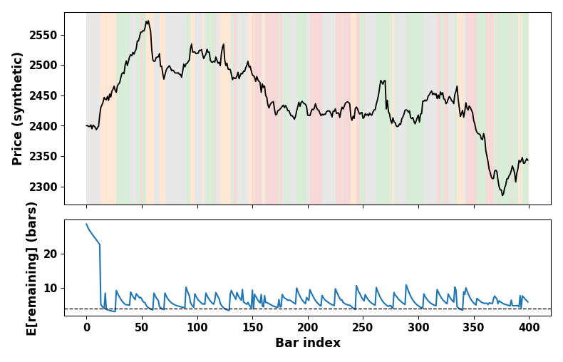
Fig. 4. Top: synthetic price path shaded by the filter's confirmed regime. Bottom: expected remaining duration for the currently favored state, with the illustrative entry threshold (4 bars) marked. Notice how the duration estimate decays toward zero near each regime transition well before the shading itself changes — that decay is the early-warning signal ManageTrades() uses for the duration-gated exit.
Visualizing the regime: the indicator's incremental filter
HSMM_RegimeIndicator.mq5 plots the same model on-chart as a color-coded regime line plus a duration histogram, loading its own independent CHSMMFilter instance from the same manifest — keeping it decoupled from the EA's own filter state so it can be attached or removed without perturbing whatever the EA is trading on.
//+------------------------------------------------------------------+
//| OnInit                                                           |
//+------------------------------------------------------------------+
int OnInit()
  {
   SetIndexBuffer(0, BufferRegimeValue, INDICATOR_DATA);
   SetIndexBuffer(1, BufferRegimeColor, INDICATOR_COLOR_INDEX);
   SetIndexBuffer(2, BufferDuration,    INDICATOR_DATA);

   ArraySetAsSeries(BufferRegimeValue, false);
   ArraySetAsSeries(BufferRegimeColor, false);
   ArraySetAsSeries(BufferDuration,    false);

   PlotIndexSetDouble(0, PLOT_EMPTY_VALUE, EMPTY_VALUE);
   PlotIndexSetDouble(1, PLOT_EMPTY_VALUE, EMPTY_VALUE);

   if(!g_ind_filter.LoadManifest(InpManifestFilename))
     {
      Print("HSMM_RegimeIndicator: manifest load/contract check failed, refusing to start.");
      return(INIT_FAILED);
     }

   g_ind_atr_handle = iATR(_Symbol, _Period, InpATRPeriod);
   if(g_ind_atr_handle == INVALID_HANDLE)
     {
      Print("HSMM_RegimeIndicator: failed to create ATR handle, err=", GetLastError());
      return(INIT_FAILED);
     }

//--- -1 is a deliberate "nothing finalized yet" sentinel, distinct
//--- from any real array index (which starts at 0), so the first
//--- OnCalculate() call can unambiguously detect the cold-start case.
   g_last_finalized_index = -1;

   IndicatorSetString(INDICATOR_SHORTNAME, "HSMM Regime (Duration-Aware)");
   return(INIT_SUCCEEDED);
  }
The real subtlety is in OnCalculate(). Most indicators can recompute any bar independently — a moving average at bar 500 does not care about bar 499. This model cannot: CHSMMFilter::StepFilter() is recursive, so MQL5's usual "resume from prev_calculated-1" pattern would re-invoke it on an already-finalized bar (most commonly the still-forming current bar, recalculated on every tick), double-counting that bar's observation and corrupting every update after it.
The fix is bookkeeping the indicator owns itself, separate from prev_calculated: g_last_finalized_index only advances once a bar has genuinely been stepped through. A full history reload resets both the belief and this counter, since the belief would otherwise no longer match the bars on the chart:
//+------------------------------------------------------------------+
//| OnCalculate                                                      |
//+------------------------------------------------------------------+
int OnCalculate(const int rates_total,
                 const int prev_calculated,
                 const datetime &time[],
                 const double &open[],
                 const double &high[],
                 const double &low[],
                 const double &close[],
                 const long &tick_volume[],
                 const long &volume[],
                 const int &spread[])
  {
//--- this indicator's model, CHSMMFilter, is RECURSIVE: each call to
//--- StepFilter() consumes exactly one bar's worth of evidence and
//--- permanently updates the belief state. That makes it fundamentally
//--- different from a typical indicator formula, which can recompute
//--- any single bar independently of the others. If we used the standard
//--- "resume from prev_calculated-1" pattern, some bars would be
//--- revisited (e.g., during recalculation of the still-forming bar).
//--- The filter would process them twice, double-counting evidence and
//--- corrupting subsequent belief updates. g_last_finalized_index
//--- is this indicator's OWN bookkeeping, kept deliberately separate
//--- from prev_calculated, and it only ever advances -- never rewinds
//--- -- once a bar has actually been stepped through the filter.
   if(rates_total < FEATURE_LOOKBACK + 2)
      return(0);   // not enough history yet to form even one feature window

//--- a full history reload (e.g. chart timeframe change, or history
//--- reload after a terminal restart) invalidates our bookkeeping --
//--- detected here as prev_calculated resetting to zero while we
//--- believe bars were already finalized. In that case the belief
//--- state itself is stale (it was built from a DIFFERENT bar
//--- sequence), so we must reset the filter's belief from scratch
//--- rather than silently continuing to step a belief that no longer
//--- corresponds to the bars actually on the chart.
   if(prev_calculated == 0 && g_last_finalized_index >= 0)
     {
      g_ind_filter.ResetBelief();
      g_last_finalized_index = -1;
     }

   int start_index;
   if(g_last_finalized_index < 0)
     {
      //--- cold start: the earliest bar with a full FEATURE_LOOKBACK
      //--- window behind it is index FEATURE_LOOKBACK (0-based,
      //--- ascending array), so pre-fill everything before that with
      //--- EMPTY_VALUE (there is simply no feature window available).
      for(int i = 0; i < FEATURE_LOOKBACK && i < rates_total; i++)
        {
         BufferRegimeValue[i] = EMPTY_VALUE;
         BufferRegimeColor[i] = 0;
         BufferDuration[i]    = EMPTY_VALUE;
        }
      start_index = FEATURE_LOOKBACK;
     }
   else
      start_index = g_last_finalized_index + 1;

//--- the LAST array index (rates_total-1) is always the still-forming
//--- bar -- we deliberately never step the filter on it, only on
//--- bars that have actually closed, so last_closed is the true upper
//--- bound for stepping.
   int last_closed = rates_total - 2;

   double atr_array[];
   ArraySetAsSeries(atr_array, false);
   int atr_needed = rates_total;
   if(CopyBuffer(g_ind_atr_handle, 0, 0, atr_needed, atr_array) < atr_needed)
      return(prev_calculated);   // ATR history not fully available yet -- try again next call

   double temp_close[];
   ArrayResize(temp_close, FEATURE_LOOKBACK + 1);

   for(int i = start_index; i <= last_closed; i++)
     {
      //--- CHSMMFilter::ComputeFeatures expects a SERIES-indexed
      //--- window (index 0 = the bar being scored, higher index =
      //--- older), but OnCalculate's close[] here is ascending. Rather
      //--- than write and maintain a second, ascending-array version
      //--- of the feature math, we copy the FEATURE_LOOKBACK+1 bars
      //--- ending at i into a small local buffer in series order and
      //--- reuse the exact same function the EA calls -- guaranteeing
      //--- the indicator's features can never silently drift out of
      //--- sync with the EA's.
      for(int k = 0; k <= FEATURE_LOOKBACK; k++)
         temp_close[k] = close[i - k];

      double features[];
      if(!g_ind_filter.ComputeFeatures(temp_close, 0, atr_array[i], features))
        {
         BufferRegimeValue[i] = (i > 0) ? BufferRegimeValue[i - 1] : EMPTY_VALUE;
         BufferRegimeColor[i] = (i > 0) ? BufferRegimeColor[i - 1] : 0;
         BufferDuration[i]    = (i > 0) ? BufferDuration[i - 1]    : EMPTY_VALUE;
         g_last_finalized_index = i;
         continue;
        }

      g_ind_filter.StepFilter(features);

      double confidence;
      int state = g_ind_filter.GetFilteredState(confidence);
      double exp_dur = g_ind_filter.GetExpectedRemainingDuration(state);

      BufferRegimeValue[i] = state;
      BufferRegimeColor[i] = state;   // color index maps 1:1 onto the four indicator_color1 entries
      BufferDuration[i]    = exp_dur;

      g_last_finalized_index = i;
     }

//--- the still-forming bar is drawn as a repeat of the last finalized
//--- value so the plotted line does not visibly drop to EMPTY_VALUE
//--- for one bar on every chart refresh -- purely cosmetic, it never
//--- touches the filter's belief state.
   if(rates_total - 1 >= 0 && last_closed >= start_index - 1 && last_closed >= 0)
     {
      int forming = rates_total - 1;
      BufferRegimeValue[forming] = BufferRegimeValue[last_closed];
      BufferRegimeColor[forming] = BufferRegimeColor[last_closed];
      BufferDuration[forming]    = BufferDuration[last_closed];
     }

   return(rates_total);
  }
The still-forming last bar is never fed through the filter — it is drawn as a repeat of the previous bar's value purely so the line does not visibly drop on every refresh, a cosmetic repeat that never touches g_ind_filter's actual belief state.
Edge cases and pitfalls
- Manifest/compile-time mismatch. If NUM_STATES, NUM_FEATURES, or MAX_DURATION changes without retraining (or vice versa), ValidateContract() is the only thing standing between a stale manifest and a corrupted belief state — treat a contract-mismatch log line as a hard stop, not a warning to investigate later.
- Belief-state edge cases: cold start and underflow. For the first several dozen bars after start, m_alpha is still near its uniform prior and the filtered state is close to arbitrary — InpConfirmBars/InpConfirmThreshold offer some protection, but do not expect a meaningful call immediately. UpdateStep() also falls back to a fresh uniform belief if the post-multiplication total collapses below 1e-300; this should only happen after an extended run of observations unlikely under every state at once, usually signaling a data anomaly or a manifest that no longer matches the instrument, not something to silently reset past.
- Truncated duration tails. Any state whose true duration distribution has meaningful mass beyond MAX_DURATION bars has that mass silently dropped in PredictStep()'s truncated loop, showing up as mild overconfidence that a long-running regime is about to end. Widening MAX_DURATION requires both a recompile and retraining.
- Feature edge cases: illiquid windows and train/live drift. A stretch of genuinely flat prices (thin session, feed outage) can drive path_sum toward its floor, pushing efficiency_ratio to a misleading extreme that the guard floors prevent from blowing up but not from feeding the model bad data. Separately, since ComputeFeatures() is shared verbatim by the EA and indicator, the only real drift risk is between this MQL5 implementation and train_hsmm.py's Python port — there is no contract check for this the way there is for array shapes, so it has to be caught by discipline.
- Hysteresis interacting with duration gating. UpdateConfirmedState() and ManageTrades()'s duration checks guard against different things and can occasionally work against each other — a genuinely short-lived regime (HighVolChop, by design) may finish before the hysteresis counter confirms it, making some short regimes effectively invisible to the trading logic despite being correctly identified. This is intentional: a regime too short-lived to confirm is also too short-lived to safely trade.
Testing in the Strategy Tester
These are real Strategy Tester results against a manifest trained on genuine XAUUSD M5 history via train_hsmm.py, not a simulation. The system was net unprofitable over this window, and that result is reported as-is.
This run covered January 1 through August 24, 2026 on XAUUSD M5 — about eight months, a single continuous stretch rather than the multi-year, multi-regime window this section originally called for. Eight months is enough for a first read, but not enough to say how this manifest behaves in a genuinely different volatility backdrop — a longer, walk-forward run across more than one window is still worth doing.
| Setting | Value |
|---|---|
| Symbol/Timeframe | XAUUSD/M5 |
| Test period | 2026.01.01 — 2026.08.24 (~8 months) |
| InpRiskPercent | 0.75% equity per trade |
| InpSL_ATR_Mult/InpTP_ATR_Mult | 2.0/4.0 |
| InpConfirmBars/InpConfirmThreshold | 3 bars/0.55 |
| InpMinEntryDuration/InpExitDuration | 4.0 bars/1.0 bars |
| Result | Value |
|---|---|
| Initial deposit/Final balance | $10,000.00 / $9,327.25 |
| Net profit | -$672.75 |
| Profit factor | 0.99 |
| Sharpe ratio/Expected payoff | -0.41 / -0.29 |
| Balance drawdown (relative) | 32.26% ($4,439.31) |
| Total trades/Total deals | 2,336 / 4,672 |
| Win rate (short/long) | 44.04% / 46.44% |
Real Strategy Tester equity curve, XAUUSD M5, Jan-Aug 2026
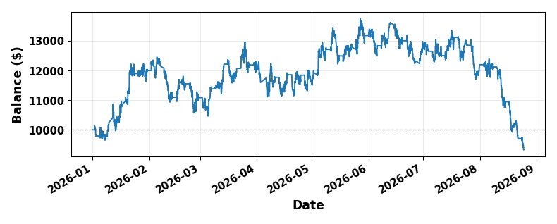
Fig. 5. Real account balance over the full 2,336-trade test, XAUUSD M5, January–August 2026. The dashed line marks the $10,000 starting balance. Balance ran up to roughly $13,760 mid-test before giving nearly all of it back, finishing modestly below the starting point.
One of the three diagnostics this section originally proposed checking can already be answered from this single run: the distribution of exit reasons. Of the 2,336 closed trades, 1,365 (58.4%) were closed by ManageTrades()'s manual duration/regime-gate path rather than by hitting a stop-loss or take-profit level, with 733 (31.4%) stopped out and 237 (10.1%) hitting take-profit. That in itself says the duration gate is not a rarely-triggered edge case — it is doing real, frequent work.
Breaking profit down by exit reason is where this result gets genuinely informative rather than just discouraging. The duration/regime-gated exits were net profitable on their own — average $16.48 per trade, a 59.3% win rate across all 1,365 of them, for a combined contribution of roughly +$22,500. Take-profit hits were unsurprisingly the strongest single category, averaging $161.17 per trade. The entire net loss for the test, and then some, traces back to the 733 stop-loss exits, which averaged -$83.72 each for a combined roughly -$61,370. In other words: the piece of this system this article set out to build —getting out of a fading trend before the state label itself flips — appears to be working and paying for itself. The piece dragging the result underwater is upstream of that, in which trades get entered and how tightly InpSL_ATR_Mult sets their stop relative to how often the emission model's regime call turns out to be wrong. That points squarely at entry filtering and stop placement as the next things to tune, rather than at the duration-awareness mechanism itself — though confirming that reading properly is exactly what the ablation run below is for, and it has not been run yet.
The other two diagnostics — average holding time versus expected remaining duration at entry, and regime-confirmation latency — need the per-bar regime log CSV (written by LogBar() during this same run) rather than just the deal list, and are not covered here yet. The natural next step, alongside a longer test window, is the ablation this section originally proposed: running the same manifest and settings with InpMinEntryDuration and InpExitDuration both set to zero, which degenerates the duration gate to a no-op and leaves only the raw state label driving entries and exits. Comparing that run's stop-loss-versus-manual-exit profit split against the numbers above would isolate, directly, how much of the positive manual-exit result is actually attributable to duration-awareness rather than to the hysteresis-confirmed state label alone.
Conclusion
The core idea here is a small one that turns out to matter more in practice than it sounds on paper: a regime's age is information. A plain HMM throws that information away by construction, folding duration into a single constant transition probability that behaves the same whether a trend just started or has been running for hours. An HSMM keeps duration as its own explicit, per-state distribution, and the payoff is a live number — expected remaining duration—that a trading system can actually act on: entering trend trades only when there is model-estimated runway left, and stepping out ahead of a reversal rather than waiting for the state label itself to flip.
Everything that runs live is native MQL5, on purpose. The manual JSON parser in CJSONArrayUtils is not a general-purpose library, it is a small, targeted tool built for exactly the manifest schema this project needs, and the forward filter in CHSMMFilter is a direct, unaccelerated implementation of the residual-time HSMM recursion — no neural network, no ONNX runtime, nothing that requires anything beyond what ships in the terminal. The only place Python enters the picture is offline, fitting parameters once via EM before they ever reach the chart.
The first real test result bears this out in a specific, checkable way rather than just in principle: across an eight-month XAUUSD M5 run, the trades closed by the duration/regime gate were net profitable (59.3% win rate, +$16.48 average), while the net loss for the system as a whole traced back almost entirely to stop-loss exits. That is a genuinely useful signal from a single test, not a conclusion — the ablation run described in Section 10 is what would confirm whether the duration gate is actually responsible for that split, or whether the hysteresis-confirmed state label alone would have produced something similar.
The most direct extension, now that a real Strategy Tester run is in hand, is exactly that ablation, followed by a longer, multi-regime test window and walk-forward re-fitting: retraining the manifest on a rolling window and comparing a periodically-refreshed model against the static one shipped here, to see how much of the edge (if any) comes from the duration-awareness itself versus simply keeping the emission model's feature statistics current. A second natural extension is adding a fifth state for genuine news-driven volatility spikes, distinguishing them from the slower-building HighVolChop state already in the model — the duration distributions for those two are likely to look very different, which is exactly the kind of thing this framework is built to represent.
If adapting to another instrument or timeframe, reconsider MAX_DURATION and FEATURE_LOOKBACK before retraining; there is no universal setting. MAX_DURATION should be set from the actual duration statistics of the instrument's regimes at the chosen timeframe — 60 bars is a reasonable starting point for XAUUSD M5, where a persistent intraday trend commonly runs several hours, but the same constant on a much higher timeframe would need to be far smaller in bar-count terms to represent a comparable wall-clock duration. FEATURE_LOOKBACK trades off responsiveness against noise in the opposite direction: a shorter window reacts faster to a genuine regime break but produces noisier efficiency-ratio and skew estimates on any instrument with lower per-bar liquidity, which in turn widens the emission Gaussians and makes every state look more alike to the filter. Both are compile-time constants precisely so that changing either one forces a conscious retrain and recompile rather than a silent runtime mismatch — the three-way contract check in Section 5 exists specifically to catch anyone who forgets one half of that pair.
| File | Type | Description |
|---|---|---|
| HSMMFilter.mqh | Include | CJSONArrayUtils (manifest parsing) and CHSMMFilter (duration-aware forward filter, feature engineering, emission scoring). |
| HSMM_RegimeEA.mq5 | Expert Advisor | Loads the manifest, steps the filter once per closed bar, applies hysteresis-confirmed regime gating, and trades with ATR-normalized position sizing and duration-gated entries/exits. |
| HSMM_RegimeIndicator.mq5 | Indicator | On-chart visualization of the filtered regime and expected remaining duration, with its own incremental, double-step-safe bookkeeping. |
| train_hsmm.py | Python (offline) | Loads MetaTrader 5-exported OHLC history, builds features identical to the MQL5 implementation, fits the HSMM via EM (forward-backward E-step, negative-binomial duration M-step), and exports hsmm_manifest.json. |
| hsmm_manifest.json | Data file | Fitted model parameters (emission means/variances, transition matrix, duration pmfs, feature normalization stats) in the schema CHSMMFilter::LoadManifest() expects. Ships here as an illustrative example structure — replace with your own trained output. |
Warning: All rights to these materials are reserved by MetaQuotes Ltd. Copying or reprinting of these materials in whole or in part is prohibited.
This article was written by a user of the site and reflects their personal views. MetaQuotes Ltd is not responsible for the accuracy of the information presented, nor for any consequences resulting from the use of the solutions, strategies or recommendations described.

 Rough Volatility: Building a Roughness Index Feature from the RFSV Model for ML Trade Filtering
 Creating a Cairo-Inspired Graphics Library for MetaTrader 5 (Part 4): Anti-Aliasing, Coverage and Compositing
 Features of Experts Advisors
 Neural Networks in Trading: A Unified View of Space and Time (Extralonger)

- Free trading apps
- Over 8,000 signals for copying
- Economic news for exploring financial markets
You agree to website policy and terms of use