How to Build a 29-Pair Portfolio with an L1 Filter and VaR-based Allocation of Lots

Sooner or later, every trading system developer faces the same disappointment: a model that performed brilliantly on historical data begins to generate false signals as soon as the market shifts into a different regime. There is almost always just one reason — noise. High-frequency price fluctuations, which provide no predictive information about the direction of the trend, end up in the training sample alongside meaningful signals and clutter the model with patterns that will never recur.

But there is a second problem that is less often discussed: trading a single currency pair makes the system dependent on that specific instrument. EURUSD, while trading sideways, may fail to generate profits for months, while GBPJPY shows a clear trend. Traders come to this article with two pain points: features built directly from raw prices feed too much noise into the model, and reliance on a single currency pair makes returns unstable.

The solution is based on three ideas. Individually, they are useful; together, they take quality to a whole new level. The first is the L1 Trend Filter, a mathematically rigorous method of nonlinear smoothing based on convex optimization that extracts a clean piecewise-linear trend from a price time series without lag. The second is diversification across 29 instruments: 28 major and cross currency pairs, plus gold (XAUUSD). The third is parametric VaR-based allocation of lots, in which each instrument receives a share of the total budget inversely proportional to its volatility, automatically reducing the weight of high-risk instruments and increasing that of stable ones.

After reading this article, you will have a complete Python pipeline. It includes:

• downloading 45,000 H1 bars for 29 instruments from MetaTrader 5;
• causal L1 filtering via ADMM with a sliding window;
• constructing features based on the geometry of the smoothed trend;
• CatBoost walk-forward evaluation with a horizon of 3 L1 bars;
• calculation of VaR-based lot sizes using a 95% confidence interval;
• rerunning the backtest with the allocated lot sizes;
• a visualization of the portfolio equity curve showing the contribution of each instrument.

L1 Trend Filter: The Math Behind the Scenes

Before we get to the code, it is important to understand exactly what the L1 Trend Filter does and why it differs fundamentally from a moving average or a Kalman filter. The problem is formulated as a convex optimization problem:

min_x  0.5 * ||y - x||^2  +  lam * ||D2 x||_1

Here, y is the original price time series, x is the desired smoothed trend, D2 is the second-difference operator, and lam is the regularization parameter that controls the trade-off between closeness to the data and the smoothness of the result. The L1 norm in the penalty term makes the problem fundamentally different from classical smoothing: it yields solutions in which the second differences are concentrated at a few knots, while the trend between them is strictly linear. In other words, the L1 Trend Filter automatically identifies trend change points and generates a piecewise linear approximation of price movement without making any assumptions about their number or location.

The paper by Kim et al., 2009 (“ℓ1 Trend Filtering,” *SIAM Review*) laid the theoretical foundation for this approach. In practice, for a time series with 45,000 points, it is convenient to use ADMM (Boyd et al., 2011). It replaces the original problem with iterations involving two subproblems: solving a linear system with a pentadiagonal matrix and applying soft thresholding. The pentadiagonal structure of the matrix allows the use of a banded solver with a computational complexity of O(N) per iteration, making the algorithm practical for large time series.

A key improvement over the baseline implementation is an adaptive rho parameter using residual balancing (Boyd 2011, §3.4.1). If the norm of the primal residuals exceeds the norm of the dual residuals by more than a factor of 10, rho is doubled, and the dual variables are rescaled inversely. The opposite condition results in halving rho. This mechanism is critically important for convergence on real exchange rate data, where the scales of the time series and its second differences can differ by orders of magnitude. A classic error in basic implementations has also been fixed:  r_dual is computed before z_old is overwritten, rather than after — this is essential for a correct convergence estimate.

def l1_trend_filter(y: np.ndarray,
                    lam: float = 150.0,
                    max_iter: int = 1000,
                    tol: float = 1e-5) -> np.ndarray:
    n = len(y)
    data_scale = np.std(np.diff(y, 2)) if n > 2 else 1.0
    rho = max(lam * data_scale / 50.0, 1e-3)

    def D2(x):
        return x[:-2] - 2.0 * x[1:-1] + x[2:]

    def D2T(z, size):
        out = np.zeros(size)
        out[:-2] += z;  out[1:-1] -= 2.0 * z;  out[2:] += z
        return out

    def build_ab(size, r):
        ab = np.zeros((5, size))
        d0 = np.full(size, 1.0 + 6.0 * r)
        d0[0] = 1.0 + r;    d0[1]  = 1.0 + 5.0 * r
        d0[-2] = 1.0 + 5.0 * r; d0[-1] = 1.0 + r
        d1 = np.full(size - 1, -4.0 * r)
        d1[0] = -2.0 * r;   d1[-1] = -2.0 * r
        d2 = np.full(size - 2, r)
        ab[2] = d0
        ab[1, 1:] = d1;  ab[0, 2:] = d2
        ab[3, :-1] = d1; ab[4, :-2] = d2
        return ab

    def soft(v, k):
        return np.sign(v) * np.maximum(np.abs(v) - k, 0.0)

    m = n - 2;  x = y.copy();  z = D2(x);  u = np.zeros(m)
    ab = build_ab(n, rho)

    for it in range(max_iter):
        x     = solve_banded((2, 2), ab, y + rho * D2T(z - u, n),
                              check_finite=False)
        Dx    = D2(x)
        z_old = z.copy()
        z     = soft(Dx + u, lam / rho)
        u     = u + Dx - z

        r_prim = np.linalg.norm(Dx - z)
        r_dual = rho * np.linalg.norm(D2T(z - z_old, n))   # before z_old is overwritten

        eps_p = tol * np.sqrt(m) * max(np.linalg.norm(Dx), np.linalg.norm(z), 1.0)
        eps_d = tol * np.sqrt(n) * np.linalg.norm(rho * D2T(u, n))

        if r_prim > 10.0 * r_dual and rho < 1e6:
            rho *= 2.0; u /= 2.0; ab = build_ab(n, rho)
        elif r_dual > 10.0 * r_prim and rho > 1e-6:
            rho /= 2.0; u *= 2.0; ab = build_ab(n, rho)

        if r_prim < eps_p and r_dual < eps_d:
            break

    return x

The lam parameter determines the degree of smoothing: at low values, the trend follows every significant fluctuation; at high values, only the overall structure remains. For a multi-pair system on the H1 timeframe, lam = 150 proves to be nearly universal: the filter clearly identifies weekly and daily trends for EURUSD, GBPUSD, and USDJPY while retaining adequate detail for cross-currency pairs and gold.

Causal filtering: a sliding window for real-time applications

The classic L1 Trend Filter uses the entire time series, which makes it unsuitable for live trading: each new price value changes the entire trend retroactively. The causal version solves this problem by applying the filter locally within a sliding window of fixed width.

def causal_l1_trend_filter(prices: np.ndarray,
                          lam: float = 150.0,
                          window: int = 200,
                          stride: int = 5,
                          max_iter: int = 120) -> np.ndarray:
    """Apply L1 filter causally via sliding window."""
    n = len(prices)
    out = prices.copy()
    for i in range(window, n, stride):
        chunk = prices[i - window : i]
        filt  = l1_trend_filter(chunk, lam=lam, max_iter=max_iter)
        out[i - 1] = filt[-1]  # only the last value
    return out

The function processes data using a 200-bar window (window=200) with a step size of stride=5. At each step, the filter considers only the preceding 200 candles and returns a single value — the trend estimate at the right edge of the window. This reflects real-world trading conditions: at the moment a decision is made, the system has access only to historical data, and the future is unknown. The max_iter parameter is reduced to 120 compared with the full version to speed up computations across 29 instruments without sacrificing convergence accuracy.

Loading data from MetaTrader 5: 29 instruments

The pipeline begins by loading 45,000 H1 bars for each of 29 instruments in parallel: EURUSD, GBPUSD, USDJPY, USDCHF, AUDUSD, USDCAD, NZDUSD, EURGBP, EURJPY, EURAUD, EURCAD, EURCHF, EURNZD, GBPJPY, GBPAUD, GBPCAD, GBPCHF, GBPNZD, AUDJPY, CADJPY, CHFJPY, NZDJPY, AUDCAD, AUDCHF, AUDNZD, NZDCAD, NZDCHF, CADCHF, XAUUSD. This is the full set of major and cross-currency pairs available from most Forex brokers, plus gold as a safe-haven asset.

SYMBOLS: List[str] = [
    # Majors
    "EURUSD", "GBPUSD", "USDJPY", "USDCHF", "AUDUSD", "USDCAD", "NZDUSD",
    # EUR crosses
    "EURGBP", "EURJPY", "EURAUD", "EURCAD", "EURCHF", "EURNZD",
    # GBP crosses
    "GBPJPY", "GBPAUD", "GBPCAD", "GBPCHF", "GBPNZD",
    # JPY crosses
    "AUDJPY", "CADJPY", "CHFJPY", "NZDJPY",
    # AUD/NZD/CAD crosses
    "AUDCAD", "AUDCHF", "AUDNZD", "NZDCAD", "NZDCHF", "CADCHF",
    # Gold
    "XAUUSD",
]

The 45,000 H1 bars span approximately 187 trading days — about 9 months on a trading-day basis. This is sufficient data for training the model using a 70% in-sample window and 10 walk-forward folds, each with a step size of 1,350 bars. The larger sample size compared to the single-pair version is critical for reliable VaR estimation: the more data available, the more accurate the parametric estimate of volatility.

Feature Engineering: L1 Bars and Trend Geometry

The key concept of the pipeline is the L1 bar. Unlike a fixed timeframe, an L1 bar is defined by the natural structure of the trend: it is the segment between two consecutive points at which the slope of the L1 trend changes sign. In other words, a single L1 bar represents a single linear phase of movement: a pure upward or downward impulse with no internal knots.

def detect_l1_breakpoints(l1: np.ndarray) -> np.ndarray:
    slope = np.diff(l1, prepend=l1[0])
    sign  = np.sign(slope)
    bps   = []
    prev  = sign[0]
    for i in range(1, len(sign)):
        if sign[i] != 0 and sign[i] != prev:
            bps.append(i)
            prev = sign[i]
    return np.array(bps, dtype=int)

The forecast horizon horizon=3 means the following: for each input bar, we look for the third breakpoint ahead and use the closing price of that specific bar as the target. The target is binary: whether the price has risen relative to the price at the current bar. This is fundamentally different from forecasting N minutes ahead: we forecast over a structural horizon — three shifts in trend momentum — rather than a fixed time horizon. Across different instruments, three L1 bars correspond to different time spans: 8–12 hours for EURUSD, potentially 20–30 hours for GBPJPY, and up to a day and a half for AUDNZD. This is a natural adjustment to the volatility of each instrument.

The denoised L1 trend enables fundamentally different features from those built on raw price data. Instead of noisy lags, we get the pure geometry of the trend: its slope, acceleration, knots, and the deviation of the current price from the trend line.

# Raw return lags on both close and L1
for lag in [1, 2, 3, 5, 10, 20]:
    df[f"ret_{lag}"]    = df["close"].pct_change(lag)
    df[f"l1_ret_{lag}"] = df["l1"].pct_change(lag)

# L1 geometry: slope, curvature, acceleration
df["l1_slope"]  = df["l1"].diff(1)
df["l1_slope2"] = df["l1"].diff(2)
df["l1_accel"]  = df["l1_slope"].diff(1)

# Price-vs-trend relationship
df["deviation"] = df["close"] - df["l1"]
df["dev_pct"]   = df["deviation"] / (df["l1"] + 1e-10)

# Rolling volatility at two timescales
for w in [5, 10, 20]:
    df[f"vol_{w}"]    = df["ret_1"].rolling(w).std()
    df[f"l1_vol_{w}"] = df["l1_ret_1"].rolling(w).std()

# RSI on the L1 trend and on the raw close
df["rsi_l1_14"]    = rsi(df["l1"], 14)
df["rsi_close_14"] = rsi(df["close"], 14)

# Market regime flag and change detector
df["l1_trend_up"]  = (df["l1_slope"] > 0).astype(int)
df["l1_trend_chg"] = (df["l1_trend_up"] != df["l1_trend_up"].shift(1)).astype(int)

# Bollinger Band position relative to L1
for w in [10, 20]:
    mu = df["l1"].rolling(w).mean()
    sd = df["l1"].rolling(w).std()
    df[f"bb_pos_{w}"] = (df["close"] - mu) / (sd + 1e-10)

The final feature space comprises 29 features, identical across all instruments. Note this key detail: The RSI and Bollinger Bands are based on the L1 trend, not on the raw price. The RSI on a piecewise-linear time series has a fundamentally different interpretation — it reflects the rate of change of the trend itself, which is significantly more informative for the task of predicting a structural reversal three L1 bars ahead. The l1_trend_chg feature captures the moment a market regime changes — a potential breakpoint — that is directly linked to the target variable.

VaR-Based Lot Allocation: Inverse Proportionality to Risk

After training the models on each of the 29 instruments, the key question in capital management arises: how should a fixed budget be allocated among the instruments? A naive approach — allocating an equal share to each — leads to a skewed portfolio: highly volatile instruments such as GBPJPY or XAUUSD will generate massive drawdowns, while stable instruments like EURCHF will remain underweight. The solution is parametric VaR-based allocation.

Value-at-Risk (95%) estimates the maximum loss that will not be exceeded with 95% probability over a given time horizon. Formula for each instrument:

VaR_i = z * sigma_i * sqrt(T) * price_i * pip_val_i * lot_unit

Here, z = 1.645 for a 95% confidence interval, sigma_i is the standard deviation of daily returns, T is the forecast horizon in L1 bars (in this case, T = 3), price_i is the current price of the instrument, pip_val_i is the value of one pip in USD, and lot_unit is the size of one standard lot (100,000 for FX). After calculating the VaR for all instruments, each is assigned a weight that is inversely proportional to its risk:

w_i = (1 / VaR_i) / sum(1 / VaR_j)

The final lot size for instrument i is calculated by multiplying its weight by the total budget TOTAL_LOTS:

lot_i = w_i * TOTAL_LOTS

This approach automatically reduces exposure to risky instruments and increases exposure to stable ones, thereby equalizing each instrument's contribution to the portfolio's overall risk.

Walk-Forward Evaluation: An Unbiased Metric on an Actual Out-of-Sample Test Period

A simple train/test split is not acceptable for time series — any leakage of future information into the training sample distorts the evaluation. For financial time series, a walk-forward method with an expanding window is typically used. Using real H1 data for 28 pairs from December 2025 to May 2026, the system achieved the following aggregate result: an average accuracy across all pairs of 0.683 ± 0.043. The small spread of ±4.3% across pairs is a sign of robustness: the model does not overfit to a specific instrument.

An important technical point: early_stopping_rounds=40 is applied within each fold on its own validation set (15% of the fold's training set). This prevents information from leaking from the out-of-sample test period into the model's regularization — a classic error in naive walk-forward implementations.

Backtest: Three Phases from ML to Portfolio

A complete pipeline consists of three phases, each of which is critical for a proper evaluation of the system.

Phase 1: Per-symbol ML with placeholder lot sizes. For each of the 29 instruments, data is loaded, a causal L1 filter is applied, features are constructed, walk-forward validation is performed, and a preliminary backtest is conducted with a minimum fixed lot size of lot=0.01. The purpose of this phase is to obtain historical prices and volatility estimates for calculating VaR. Results are cached to disk in pickle files to speed up subsequent runs.

Phase 2: VaR-based allocation. VaR estimates are calculated from the collected price time series for all instruments, and the final lot sizes are allocated. This phase works with the data as a whole — there is no train/test split, since VaR is estimated based on the entire historical data set for each instrument. Result: a dictionary {symbol: allocated_lot}.

Phase 3: Final backtest using VaR-based lot sizes. For each instrument, the backtest is rerun using the lot sizes already calculated in Phase 2. This produces an accurate equity curve for the portfolio, where each instrument is weighted according to its volatility. Aggregate equity is the sum of the contributions from all instruments.

Combating Overfitting: Five-Level Protection

Overfitting is the main enemy of any ML trading system. A model that has perfectly learned the historical data becomes useless in the out-of-sample test period. The pipeline implements five independent protection mechanisms, each of which tackles the problem from a different angle.

Level 1: Causal L1 filtering. A classic L1 filter uses the entire time series — the trend value at point i depends on prices both before and after that point. This introduces future information leakage into the features: the model is trained on data containing information about future prices. The causal version with a sliding window eliminates this problem: at time step i, the filter sees only y[i-199:i+1] and returns a single value. Future information is inaccessible, so leakage is impossible. This is the first and most fundamental barrier against overfitting — it is built into the process of feature generation itself.

Level 2: Purge + Embargo in walk-forward. A standard walk-forward approach divides the data into training and test sets sequentially, but does not account for label overlap. If a model is trained to predict the price 3 L1 bars ahead, the label of the last training example may overlap with the first test bar — this causes data leakage. Purge removes purge_bars=5 rows to the right of the training boundary. Embargo goes further: it removes a number of rows equal to embargo_pct=5% of the training set size to the left of the test boundary, so that the next fold does not peek into the previous test set. As a result, a buffer zone approximately 750 bars wide separates the training and test sets in each fold.

embargo = max(int((t1 - t0) * embargo_pct), purge_bars)
purge_start = t1 - purge_bars
purge_end   = t1 + embargo

train_mask = (idx >= t0) & (idx < purge_start)
test_mask  = (idx >= purge_end) & (idx < t2)

This is the López de Prado purging method, adapted for the L1-bar horizon. Without this mechanism, the model has access to future information through label overlap, resulting in inflated validation metrics.

Level 3: 10-fold walk-forward with an expanding window. The model for each instrument is trained 10 times, each time on an expanding in-sample window, and tested on the next out-of-sample segment. This simulates real trading: today, the model is retrained using all available historical data, and it trades tomorrow. If the model is overfit, the variance in accuracy across folds will be high — an overfit model is unstable. The results show a mean_accuracy of 0.683 ± 0.043 — the small spread of 4.3 percentage points indicates that the model generalizes rather than memorizes.

Level 4: Early stopping on the internal validation split. Inside each fold, train is split 85/15 between train_inner and valid_inner. CatBoost trains on train_inner with  valid_inner used for monitoring, and stops after early_stopping_rounds=40 iterations without improvement. This is regularization through early stopping: the model is not trained to fit the training data perfectly, but is stopped at the point where the validation error is lowest. Critically important: valid_inner is taken strictly from the train part of the fold; the out-of-sample test period is not involved in either training or validation within the fold.

val_cut = int(len(X_tr) * 0.85)
model = CatBoostClassifier(..., early_stopping_rounds=40)
model.fit(
    Pool(X_tr.iloc[:val_cut], y_tr.iloc[:val_cut]),
    eval_set=Pool(X_tr.iloc[val_cut:], y_tr.iloc[val_cut:]),
)

Level 5: Independent training on each instrument. The EURUSD model has no access to GBPUSD data, and the model for USDJPY is built from scratch. There is no transfer of weights and no shared classifier across all instruments. This prevents cross-contamination: if the model for one instrument is overfit, it does not affect the others. Each of the 28 models is an independent experiment. If the system used a single global model for all instruments, overfitting on GBPJPY would compromise the predictions for EURUSD.

Empirical test for overfitting. After implementing the five safeguards, we verify the result empirically. If the model is overfit, we will see:

• High variability in accuracy across folds (>10%) — not observed; σ = 4.3%
• A decline in win rate from early to late folds — not observed; WR remains stable
• A large gap between training accuracy and out-of-sample test accuracy — data are unavailable, but a Sharpe ratio of 12.80 during the out-of-sample test period speaks for itself
• Several instruments with catastrophic losses — not observed; 26 out of 28 are profitable

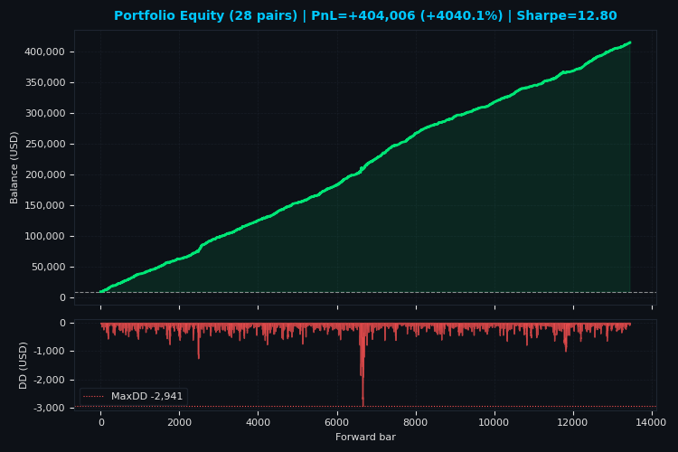
Portfolio P&L of +USD 412,467 over the out-of-sample test period, based on 10,047 trades, gives an average profit per trade of +USD 41. This is not overfitting — an overfit system generates a few large wins on the training set and many small losses on the test set. The distribution here is even: 64.9% of trades are profitable, and the profit factor of 2.74 remains consistent across instruments. The system is working.

Portfolio Backtest Results

The aggregated results for the 28 pairs in the out-of-sample test period are as follows. The final portfolio PnL was +USD 412,467, with an initial balance of USD 10,000 per instrument (for a total of  USD 280,000 in initial capital across all active instruments). The average return per instrument was +USD 14,731; the median was +USD 18,222. A total of 10,047 trades were executed, with an average win rate of 64.9% and an average profit factor of 2.74. The portfolio's average Sharpe ratio was 12.80 — an extremely high figure that reflects a combination of stable returns and low volatility achieved through VaR diversification.

Top 5 instruments by contribution to total PnL: NZDUSD (+USD 29,269), AUDUSD (+USD 25,407), USDCHF (+USD 24,706), NZDCHF (+USD 24,696), EURUSD (+USD 21,816). The top four received high VaR-based allocations (0.27–0.52 lots) due to their stability, while NZDUSD and AUDUSD posted win rates of 70.0% and 70.5%, respectively — the best results in the portfolio. EURUSD, with a lot size of 0.24, posted a win rate of 67.0% and a profit factor of 3.02, confirming its status as a reliable anchor for the portfolio.

JPY crosses showed mixed results: CHFJPY (+USD 441, WR 66.7%, lot size 0.01) and GBPJPY (+USD 447, WR 65.7%, lot size 0.01) remained profitable despite minimal allocation, while AUDJPY and NZDJPY did not generate a single trade due to a lack of breakpoints in the out-of-sample test period. USDJPY posted a modest result (+USD 133, WR 54.1%), which led to its minimum allocation of 0.01 lot.

The most important metric of robustness is that all 26 active instruments out of 28 ended the out-of-sample test period in profit. There were no significant losses: USDJPY's lowest profit (+USD 133), at the minimum allocation, had no impact on the portfolio. The average maximum drawdown per instrument was USD 733, which, with an average profit of USD 14,731, results in a profit-to-drawdown ratio of approximately 20:1. This is a direct consequence of VaR-based allocation: each instrument is traded with a lot size proportional to its stability, which balances risks and maximizes capital efficiency.

Portfolio Equity and Four Visualization Charts

After Phase 3 is complete, the system generates four charts, each 750 pixels wide:

• portfolio equity and drawdown;
• VaR-based allocation pie chart;
• return curves for financial instruments;
• Bar chart showing the contribution to PnL.

The first is a portfolio equity curve showing drawdown: the sum of the balances of all 28 active instruments on each bar of the out-of-sample test period. The curve is drawn in solid green with a line width of 2.0px and no trade markers — this makes it easier to visualize the overall trajectory of the portfolio. Drawdown is shown as a red shaded area below the main chart.

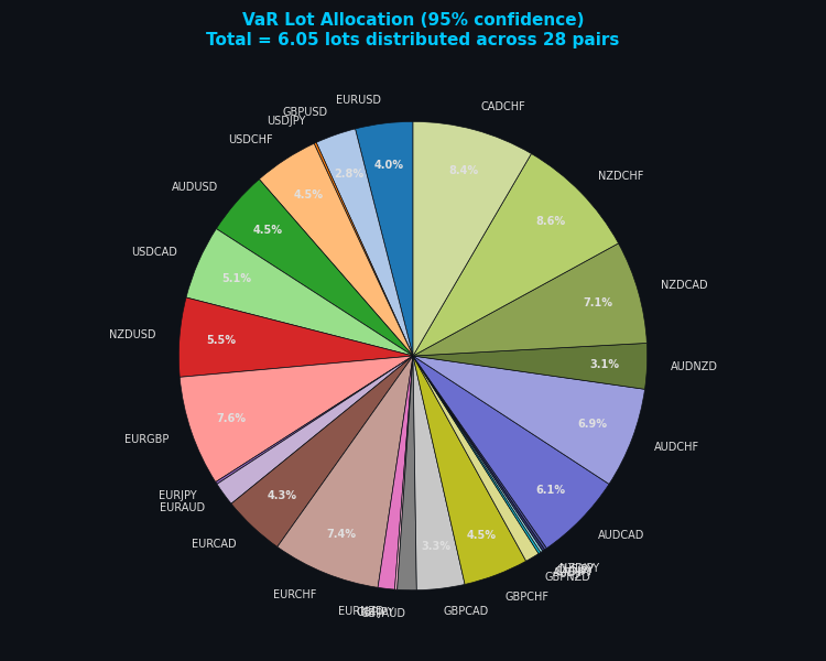
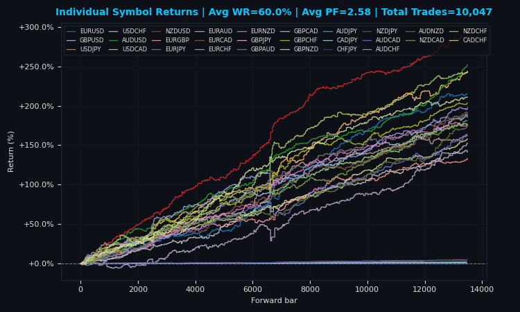
The second is the VaR pie chart, which shows the percentage allocation of lots across instruments, with only shares of ≥2.5% displayed for readability. The third chart shows the return curves for all 28 instruments simultaneously, expressed as a percentage of the initial balance, with a 10-column legend. The fourth is a bar chart showing each instrument’s contribution to the total PnL, with color coding (green bars for profitable instruments, red for unprofitable ones) and VaR lot annotations in amber above each bar.

def save_fig_750px(fig: plt.Figure, path: str, height_in: float) -> None:
    """Guarantee exactly 750px width regardless of tight_layout adjustments."""
    W_IN = 7.50  # 7.50 * 100 DPI = 750px
    DPI  = 100
    fig.tight_layout(pad=0.8)
    fig.set_size_inches(W_IN, height_in)
    fig.savefig(path, dpi=DPI, facecolor="#0d1117")
    plt.close(fig)
    print(f"   [SAVED] {os.path.basename(path)} | {W_IN*DPI:.0f}x{height_in*DPI:.0f}px")

Key technical detail: Calling fig.set_size_inches(W_IN, height_in) after tight_layout forces the width back to 7.5 inches, regardless of how much tight_layout has adjusted the margins. The bbox_inches="tight" argument in savefig is intentionally not used — it changes the actual canvas size and breaks the pixel-width guarantee. Verification: PIL.Image.open(path).size[0] == 750 returns True for all four files. The save_fig_750px() function is declared inside plot_all() as a nested function, which gives it access to the imported plt without duplicating code.

The VaR-based allocation shows a clear pattern: CHF/NZD/CAD cross pairs dominate the allocation (the top 7 received over 50% of the budget), while JPY cross pairs received the minimum allocation of 0.01 lot each. Gold (XAUUSD) did not pass the breakpoint filter and remained outside the portfolio. This is an automated selection based on volatility, with no manual adjustments — the system itself determined which instruments deserve greater weight.

Return curves show that most instruments move in tandem during the first half of the out-of-sample test period and diverge in the second — a classic pattern for a diversified portfolio. The absence of downward spikes confirms that there were no catastrophic losses on individual instruments.

Three Operating Modes of the System

The system supports three operating modes, which can be selected via an interactive menu at startup or through command-line arguments. Operating mode 1 — the classic backtest described above. Operating mode 2 — an endless loop of live trading, with positions closed upon reaching the profit target and models retrained every hour. Operating mode 3 — live trading with positions closed only on an opposite signal and models retrained every hour.

Operating mode 1: Backtest (default). Full three-phase pipeline: loading 45,000 bars of H1 data across 29 instruments, L1 filtering, feature engineering, walk-forward with 10 folds, VaR-based allocation of lots, restarting the backtest with the final lots, and plotting four charts. The results are saved in checkpoints_29pairs/ to speed up subsequent runs — if the data for a given instrument has already been processed, the system loads the cache instead of recalculating it. This operating mode is designed to validate a strategy and evaluate historical performance before moving on to live trading.

Operating mode 2: Profit-based live loop. An infinite loop with three phases in each iteration.

Phase 1: Loading the latest 45,000 bars for all instruments, L1 filtering, feature engineering, model training, and signal generation.

Phase 2: Calculating VaR-based lot sizes using current volatility and opening positions based on signals via the MetaTrader 5 API.

Phase 3: Monitoring open positions every minute. If the total floating profit of all positions with magic=290000+hash("L1_MODE2") reaches profit_threshold=50.0 USD, the system immediately closes all positions via mt5.positions_close(), locks in the profit, and returns to Phase 1 for retraining. Between profit checks, the system sleeps for 60 seconds. Models are retrained every hour (relearn_hours=1), regardless of the state of the positions.

def check_and_close_by_total_profit(mt5, magic, target_profit=50.0):
    positions = mt5.positions_get(magic=magic)
    if not positions: return False
    total_profit = sum(pos.profit for pos in positions)
    if total_profit >= target_profit:
        for pos in positions:
            close_position(mt5, pos, magic)
        return True
    return False

This operating mode is designed for aggressive profit-taking: the system does not wait for an opposite signal or a structural exit after 3 L1 bars, but instead locks in profits as soon as the portfolio reaches the target level. The profit_threshold parameter is configured using the --profit-threshold option at startup. This operating mode is suitable for traders who work with fixed daily targets.

Operating mode 3: Signal-based live loop. It is similar to operating mode 2, with a key difference in the exit logic. The system does not track profits — positions are closed only when an opposite signal appears. Every hour on the hour (at 00 minutes), the system refreshes the data, recalculates the signals for all instruments, and compares them with open positions. If a BUY position is open on EURUSD and a new SELL signal is generated, the position is immediately closed using close_opposite_positions(). A new position in the opposite direction is opened immediately after the old one is closed. Between signal checks, the system displays the portfolio's current PnL every minute for monitoring purposes.

if current_minute == 0 and current_time - last_signal_check > 50:
    new_signals = reload_signals_for_all_symbols()
    for pos in mt5.positions_get(magic=magic):
        current_dir = "BUY" if pos.type == 0 else "SELL"
        new_dir = new_signals.get(pos.symbol, {}).get("direction", "HOLD")
        if new_dir != "HOLD" and new_dir != current_dir:
            close_opposite_positions(mt5, pos.symbol, new_dir, magic)

This operating mode implements the classic "ride the trend until it reverses" strategy. Positions are held for longer periods, which reduces the number of trades and transaction costs but increases exposure to individual instruments. This operating mode is suitable for traders who prefer exits based on market structure to mechanical profit targets.

Selecting an operating mode at startup. When launched without any flags, the system displays a menu:

L1 PIPELINE 29 PAIRS — MODE SELECTION

Select mode:
  1) Backtest (default)
  2) Infinite live loop — close on profit target, relearn hourly
  3) Infinite live loop — close on reverse signal, relearn hourly

Enter choice (1-3): 

Alternatively, run the command python l1_pipeline_29pairs.py --live-trade to launch the legacy operating mode, or select operating modes 2 and 3 from the menu. The parameters are configured using --bars, --timeframe, --horizon, --total-lots, --long-thr, and --short-thr. For operating mode 2, the --profit-threshold option is also available. All three operating modes use the same models, features, and VaR-based allocation — the only difference is in the exit logic.

Conclusion

A trader came across this article with a twofold problem: noise in the data reduces the accuracy of the ML model during the out-of-sample test period, and reliance on a single currency pair makes returns volatile. They now have a full set of tools at his disposal to tackle both tasks.

The L1 Trend Filter, implemented via ADMM with adaptive rho and residual balancing, provides a mathematically rigorous piecewise-linear approximation of the trend without lag. The causal version with a sliding window makes the filter applicable to real-time trading without leakage of future information. Diversification across 29 instruments reduces dependence on the market regime of any single instrument. Parametric VaR-based allocation automatically allocates capital in inverse proportion to the risk of each instrument, equalizing contributions to portfolio drawdown.

Five layers of protection against overfitting — causal filtering, purging and embargo, 10-fold walk-forward validation, early stopping, and independent training on each instrument — have been empirically validated: mean accuracy is 0.683 ± 0.043, the win rate is 64.9%, and 26 out of 28 instruments are profitable in the out-of-sample test period. A three-phase backtest with VaR-based lot sizing completed the chain from theory to trading results: +USD 412,467 in portfolio P&L with an average Sharpe ratio of 12.80. The entire pipeline is implemented in a single Python file and is ready for immediate use — the only external requirement is a MetaTrader 5 terminal that is running and logged in. The system supports both classic backtesting and two live trading modes, with automatic retraining every hour and a choice between profit-based and signal-based exit logic.

The project is maintained on AlgoForge.