

Online False Discovery Rate Control: Putting an Error Budget on a Live Signal Stream
 378
 0

Introduction
Open a multi-timeframe scanner across 28 symbols and 7 timeframes and you have asked the market 196 questions. If each cell reports "significant at 5%", then on pure noise, with no edge anywhere on the board, roughly ten of those cells light up. Every sweep. Run it weekly and the scanner hands you five hundred confident signals a year that were never there.
The same arithmetic runs inside a single Expert Advisor. A rule that fires forty times a month at a 5% threshold produces two false alarms a month by construction, and the ones that looked strongest are the ones you deploy. When they die, the rule did not stop working. It never worked: you were reading the tail of a distribution you generated yourself.
This is the multiple testing problem, and it has a mature literature. Most of that literature is offline: gather all N results, sort them, correct once. The Deflated Sharpe Ratio and the backtest-overfitting batteries work this way, and they are excellent at the question they answer. They fit this one only with a compromise, because they need N in advance and assume every decision can be revisited after the whole batch is in. Re-running them over rolling or fixed batches works for research that can wait, but not for a decision that has to be made the moment a signal arrives. A live signal stream has no N: it never ends, the questions arrive one at a time, and each answer is acted on before the next question exists.
Online false discovery rate control is designed for this setting. Instead of a fixed threshold it maintains an error budget, spends a little on every hypothesis it examines, and is refunded on every discovery. The guarantee is specific: provided the p-values are valid, among the signals you acted on, the expected fraction that were noise stays below a level you chose. It can be checked directly only where the truth is known, which is why every procedure here is tested on synthetic data before it meets a market.
In this article we port three procedures from that literature into pure MQL5: LORD3, LORD++ and SAFFRON. Alongside them we build the machinery they need on a chart: a bank of signal rules that produce a genuine stream, a causal bootstrap p-value source, benches that establish correctness before any market data is involved, an indicator that draws the budget as it drains, and an Expert Advisor that runs the gate against its own control arm. Along the way we will find two ways this fails silently while looking healthy, and measure exactly where the guarantee stops holding.
We will cover:
- The Scanner That Cries Wolf
- Alpha-Wealth and Three Procedures
- Where the P-Values Come From
- Calibration Before the Market
- Where the Guarantee Breaks
- Watching the Budget Drain
- The Gate Under Execution
- Conclusion
The Scanner That Cries Wolf
Fix the vocabulary first, because the rest of the article depends on three terms being kept apart. A hypothesis is one question with a yes-or-no answer: at the moment this rule fires on this instrument, has it been selecting bars that precede a better-than-chance return over the next h bars? The p-value answers it from the rule's own recent firings, so it is a question about the rule's record up to now, not a forecast that this particular firing will pay. Throughout the article h is the forward horizon, the number of bars a firing is judged over, and every run shown here uses h = 10 on H1. A discovery is a hypothesis you decided to answer yes. A false discovery is a yes that was wrong. The false discovery rate is the expected value of the fraction of your discoveries that are false. A false discovery is a statement about the hypothesis, not about a trade: a true discovery can still lose money, and a false one can win.
Note what the FDR is not: it is not the probability of making any mistake at all. That stricter quantity is the family-wise error rate, and controlling it on a long stream drives the levels so low that power collapses: only very strong effects get through, as the Bonferroni rows later show. FDR tolerates a known share of mistakes among the signals you act on, in exchange for still being able to find things.
The distinction that motivates this article is between offline and online.
| Question | Offline (Benjamini-Hochberg, Deflated Sharpe, PBO) | Online (LORD, SAFFRON) |
|---|---|---|
| When is the decision made? | After every result is in hand | The moment each hypothesis arrives |
| Is the number of tests known? | Yes, you counted your trials | No, the stream never ends |
| Can a decision be revised? | Yes, the whole batch is re-thresholded | No, it is irrevocable |
| What is controlled? | FDR over the finished batch, or the inflation of one selected statistic | Noise fraction of everything acted on |
An offline method asked about a live scanner has nothing to sort: by the time the batch is complete you have already traded it. That gap is the whole opening for the online family.

Fig. 1. A 28-by-7 scanner grid tested at 5% on data with no edge. Roughly ten cells light up per sweep, and the count of accumulated false discoveries grows without limit.
Alpha-Wealth and Three Procedures
The central object is a budget. The procedure starts with an initial alpha-wealth w0, pays out the test level alpha_t for every hypothesis it examines, and is refunded a payout each time it rejects: alpha for every discovery except the first, which is worth only alpha - w0 because w0 was already advanced against it up front. Discoveries finance further testing; a long run of nulls starves the procedure. That starvation is correct behaviour rather than a defect, and it is the most important practical fact about running these procedures on a fast stream.
What turns wealth into a level is the gamma sequence: a non-increasing, non-negative sequence summing to at most one. It is the only real tuning knob, and it decides how fast the budget drains while nothing is being found. The vocabulary header defines the procedures, the configuration and that sequence.
//+------------------------------------------------------------------+
//| Which procedure assigns the test levels. The two baselines are   |
//| not filler: without them there is no way to show what the        |
//| corrected procedures actually buy.                               |
//+------------------------------------------------------------------+
enum ENUM_FDR_RULE
  {
   FDR_UNCORRECTED,        // alpha_t = alpha forever; controls nothing
   FDR_BONFERRONI,         // alpha_t = alpha*gamma_t; FWER, no refunds
   FDR_LORD3,              // level from wealth at the last rejection
   FDR_LORDPP,             // LORD++, level from the rejection history
   FDR_SAFFRON             // LORD++ that tests candidates for free
  };
The two baselines earn their place, because without them a table of FDR numbers has no scale. Uncorrected is what a scanner reporting "significant at 5%" on every cell is silently doing. Online Bonferroni divides the budget up front by the gamma sequence and never refunds it, which controls the family-wise error rate and goes quiet almost immediately.
//+------------------------------------------------------------------+
//| Everything a procedure needs to be reproducible from scratch.    |
//| w0 is kept below alpha: the first discovery refunds alpha - w0,  |
//| nothing at w0 = alpha, though later discoveries still pay alpha. |
//+------------------------------------------------------------------+
struct SFdrConfig
  {
   double            alpha;        // target FDR level
   double            w0;           // initial alpha-wealth, w0 < alpha
   double            lambda;       // SAFFRON candidate threshold
   ENUM_FDR_GAMMA    gamma;        // discount sequence
  };
Two shapes of that sequence ship, and which one you pick changes how long the procedure stays solvent, not whether it is correct.
//+------------------------------------------------------------------+
//| Shape of the gamma sequence.                                     |
//+------------------------------------------------------------------+
enum ENUM_FDR_GAMMA
  {
   FDR_GAMMA_LORD,         // Javanmard-Montanari default, sums to ~1
   FDR_GAMMA_ZETA          // j^-1.6 / zeta(1.6), sums to exactly 1
  };
FDR_GAMMA_LORD is the sequence the LORD paper defines, and it produced every number in this article. FDR_GAMMA_ZETA is the bare power law j^-1.6 divided by zeta(1.6), about 2.2856. The difference between them is entirely in where each puts its budget.
| Term | LORD | ZETA |
|---|---|---|
| gamma_1 | 0.0500 | 0.4375 |
| gamma_20 | 0.00192 | 0.00363 |
| gamma_100 | 0.000389 | 0.000276 |
| sum of first 20 | 0.132 | 0.881 |
| sum of first 2000 | 0.305 | 0.992 |
ZETA is front-loaded. It puts 88% of its allowance into the first twenty terms, so it tests at levels roughly nine times higher than LORD at the start and can still reject something before the budget is gone. The price is a thin tail: past the sixtieth term its levels fall below LORD's and keep falling, so a stream that stays quiet for a few hundred hypotheses starves harder under ZETA. LORD is the opposite trade, holding most of its allowance in reserve.
One consequence carries into the results. Both forms sum to one over an unbounded stream, but the LORD form gets there extremely slowly: after the 2000 hypotheses of the synthetic bench it has paid out only 0.305 of its total, and even after a million terms it is still short of a half. On any stream of practical length it commits a fraction of what it is allowed, and that conservatism shows up later: a large part of LORD++'s gap to target is the gamma sequence, not the procedure.
//+------------------------------------------------------------------+
//| The j-th term of the discount sequence, j >= 1. The LORD form is |
//| reproduced with the papers' own constant rather than tidied up:  |
//| that constant is what makes the series sum to one.               |
//+------------------------------------------------------------------+
double FdrGamma(const ENUM_FDR_GAMMA kind,const int j)
  {
   if(j<1)
      return(0.0);

   if(kind==FDR_GAMMA_ZETA)
      return(MathPow((double)j,-1.6)/FDR_ZETA16);

//--- log(1) is zero, so the exp() factor is one at j = 1 and the
//--- max(j,2) guards only the numerator.
   double num=MathLog((double)MathMax(j,2));
   double den=(double)j*MathExp(MathSqrt(MathLog((double)j)));
   return(0.0722*num/den);
  }
All five procedures share one base class. The bookkeeping is identical in every case: count the arrival, charge the budget, record the rejection. Only the level rule differs, so it is the only thing subclasses replace.
//+------------------------------------------------------------------+
//| Test one arriving hypothesis and record what happened.           |
//|                                                                  |
//|  Order matters here. The level is fixed before the candidate     |
//|  counter is touched, because SAFFRON's index shift is defined    |
//|  over hypotheses 1..t-1 and would otherwise include the arrival  |
//|  it is about to price.                                           |
//+------------------------------------------------------------------+
bool CFdrBase::Submit(const double p,SFdrDecision &d)
  {
   if(p<0.0 || p>1.0)
      return(false);

   m_t++;
   double lvl=Level(m_t);
   if(lvl<0.0)
      lvl=0.0;
   if(lvl>1.0)
      lvl=1.0;

   bool rej=(p<lvl);
   m_spent+=lvl;

   if(p<m_cfg.lambda)
      m_ncand++;

   if(rej)
     {
      m_earned+=Payout();
      int n=ArraySize(m_rej_t);
      ArrayResize(m_rej_t,n+1,256);
      ArrayResize(m_rej_wealth,n+1,256);
      ArrayResize(m_rej_cand,n+1,256);
      m_rej_t[n]=m_t;
      m_nrej++;
      m_rej_wealth[n]=Wealth();
      m_rej_cand[n]=m_ncand;
     }

   d.index   =m_t;
   d.p       =p;
   d.level   =lvl;
   d.rejected=rej;
   d.wealth  =Wealth();
   return(true);
  }
Two one-line accessors from the same class carry the entire budget story, and everything this article later claims about starvation is read off them.
//--- payout for the NEXT rejection. The first one is worth less
//--- because w0 was already advanced against it up front.
   double            Payout(void)      { return((m_nrej==0)?m_cfg.alpha-m_cfg.w0:m_cfg.alpha); }
The wealth is what was put in, minus everything charged, plus everything refunded. That identity is the shared ledger for all five procedures. LORD3 builds its level from it; LORD++ and SAFFRON compute their levels from the rejection history directly, so for them it is a record rather than an input. For SAFFRON it is also not the paper's own accounting, which charges only non-candidates: the panel uses the one ledger for every procedure so that their curves compare.
double Wealth(void) { return(m_cfg.w0-m_spent+m_earned); }

Fig. 2. The budget mechanism. Each examined hypothesis subtracts its level from the wealth; each discovery refunds a payout, and the level tracks the wealth back up.
LORD++ prices the next test off the entire rejection history, every past discovery still contributing but decayed by how long ago it happened. In the paper's own notation, the level is gamma_t times w0, plus (alpha - w0) times gamma indexed at the gap since the first rejection, plus alpha times the same term summed over every later rejection.
//+------------------------------------------------------------------+
//| gamma_t*w0 + (alpha-w0)*gamma_{t-tau_1} + alpha*sum_{j>=2} ...   |
//+------------------------------------------------------------------+
double CFdrLordPP::Level(const int t)
  {
   double lvl=Gamma(t)*m_cfg.w0;
   int    n  =ArraySize(m_rej_t);

   for(int j=0;j<n;j++)
     {
      int idx=t-m_rej_t[j];
      if(idx<1)
         continue;
      double payout=(j==0)?m_cfg.alpha-m_cfg.w0:m_cfg.alpha;
      lvl+=payout*Gamma(idx);
     }
   return(lvl);
  }
SAFFRON is that same sum with one change, and the change is its entire idea. A hypothesis whose p-value came back below lambda is a candidate, and SAFFRON tests candidates for free: it advances the gamma index only on non-candidates, the hypotheses with p at or above lambda, so a run of promising p-values leaves the level where it was. The whole sum is scaled by (1 - lambda) to pay for the privilege.
//+------------------------------------------------------------------+
//| The candidate counts are the point. C0 is every candidate among  |
//| hypotheses 1..t-1, so t-C0 is one more than the number of        |
//| NON-candidates, and the sequence therefore stands still while a  |
//| run of candidates streams past. Each rejection term is shifted   |
//| the same way over its own suffix of the stream.                  |
//+------------------------------------------------------------------+
double CFdrSaffron::Level(const int t)
  {
   int c0=m_ncand;

   int idx0=t-c0;
   double lvl=(idx0>=1)?Gamma(idx0)*m_cfg.w0:0.0;

   int n=ArraySize(m_rej_t);
   for(int j=0;j<n;j++)
     {
      int cj =c0-m_rej_cand[j];
      int idx=t-m_rej_t[j]-cj;
      if(idx<1)
         continue;
      double payout=(j==0)?m_cfg.alpha-m_cfg.w0:m_cfg.alpha;
      lvl+=payout*Gamma(idx);
     }

   lvl*=(1.0-m_cfg.lambda);
   return(MathMin(m_cfg.lambda,lvl));
  }
The final MathMin is a hard cap at lambda, there for consistency rather than safety: SAFFRON has already classed a p-value at or above lambda as a non-candidate, evidence for the null, so setting a bar high enough to reject one would contradict the classification the rest of the procedure rests on.

Fig. 3. SAFFRON's index shift. Only a clearly-null p-value advances the discount sequence, so a run of promising hypotheses does not drive the level down.
LORD3, the third procedure, is the most compact of the three: its level is gamma indexed at the gap since the last rejection, multiplied by the wealth that survived that rejection. Everything earlier is carried implicitly in that one wealth figure.
//+------------------------------------------------------------------+
//| gamma_{t-tau} * W(tau), with tau = 0 and W = w0 before the first |
//| rejection.                                                       |
//+------------------------------------------------------------------+
double CFdrLord3::Level(const int t)
  {
   int    tau=0;
   double w  =m_cfg.w0;
   int    n  =ArraySize(m_rej_t);
   if(n>0)
     {
      tau=m_rej_t[n-1];
      w  =m_rej_wealth[n-1];
     }

   int j=t-tau;
   if(j<1)
      return(0.0);
   return(Gamma(j)*w);
  }
That single read of the wealth recorded at the last rejection is the whole procedure, and it is also where it is brittle. LORD++ and SAFFRON price today off the entire rejection history, so one fortunate rejection is diluted by everything around it; LORD3 prices today off one number produced at one moment. When the p-values correlate, that moment can be a fluke, and the dependence experiments measure what the shortcut costs.
Where the P-Values Come From
This is the part a port can most easily get wrong. An FDR procedure controls the false discovery fraction only if the p-values it is fed are valid. Feed it a statistic that is merely small when the signal looks good and the guarantee evaporates in silence, with the arithmetic still running and the panel still drawing a plausible wealth curve.
The stream is firings, not bars. Testing every bar would submit a hundred thousand near-identical questions, and one firing of one rule is the smallest unit that is genuinely a fresh question. Five rules ship, and they are deliberately heterogeneous.
//--- the rules, in the order they are offered to the procedure
//--- whenever more than one fires on the same bar.
enum ENUM_FDR_SIGNAL
  {
   FDR_SIG_MACROSS=0,      // fast/slow moving average cross
   FDR_SIG_REVERSION,      // close leaves a z-score band
   FDR_SIG_BREAKOUT,       // close clears a rolling extreme
   FDR_SIG_MOMENTUM,       // n-bar return crosses a threshold
   FDR_SIG_VOLSQUEEZE,     // volatility drops into its low quantile
   FDR_SIG_COUNT
  };
Two trend rules, one mean-reverting, one breakout, one volatility state. Five variations of one idea would produce duplicates, and duplicates do not merely waste budget: they break the independence the procedures' proofs assume. Whether that pushes the realised FDR above the nominal one depends on the form the dependence takes, and the dependence bench later finds that correlated copies can, while plain repetition mostly costs power. Every rule computes from the close array directly rather than through indicator handles, so a run is deterministic. Each fires on a transition rather than on a state, which matters more than it looks.
//+------------------------------------------------------------------+
//| Fires on the bar the fast average changes side, not on every bar |
//| it stays there. A state rule would fire thousands of times and   |
//| every firing after the first would be a near-duplicate question. |
//+------------------------------------------------------------------+
void CSignalBank::BuildMaCross(const double &c[],const int from)
  {
   for(int i=from;i<m_total;i++)
     {
      double f0=Mean(c,i,m_ma_fast),   s0=Mean(c,i,m_ma_slow);
      double f1=Mean(c,i-1,m_ma_fast), s1=Mean(c,i-1,m_ma_slow);

      if(f1<=s1 && f0>s0)
         Set(FDR_SIG_MACROSS,i,1);
      if(f1>=s1 && f0<s0)
         Set(FDR_SIG_MACROSS,i,-1);
     }
  }
A state rule ("fast is above slow") would fire on thousands of consecutive bars, every firing after the first asking nearly the same question again: each has its own forward window, but the windows overlap almost entirely.
Two windows that must not touch
For a firing at bar i, the null under test is narrow and specific: the bars this rule selects carry no more forward return than bars picked without reference to it. The observed statistic is the mean h-bar forward return over the rule's own past firings, signed by the direction each one took.
Two windows are in play, and keeping them apart is the whole of the causality argument. The evidence window runs from lo to i-h-1, so every firing inside it has a fully observed h-bar forward return by the time bar i arrives and the p-value could genuinely have been computed there. The outcome window is bar i itself, whose forward return spans i to i+h and is strictly later than every bar the p-value saw. Without that separation the gate would be scored on the same returns that set its own threshold, and any procedure would look excellent.
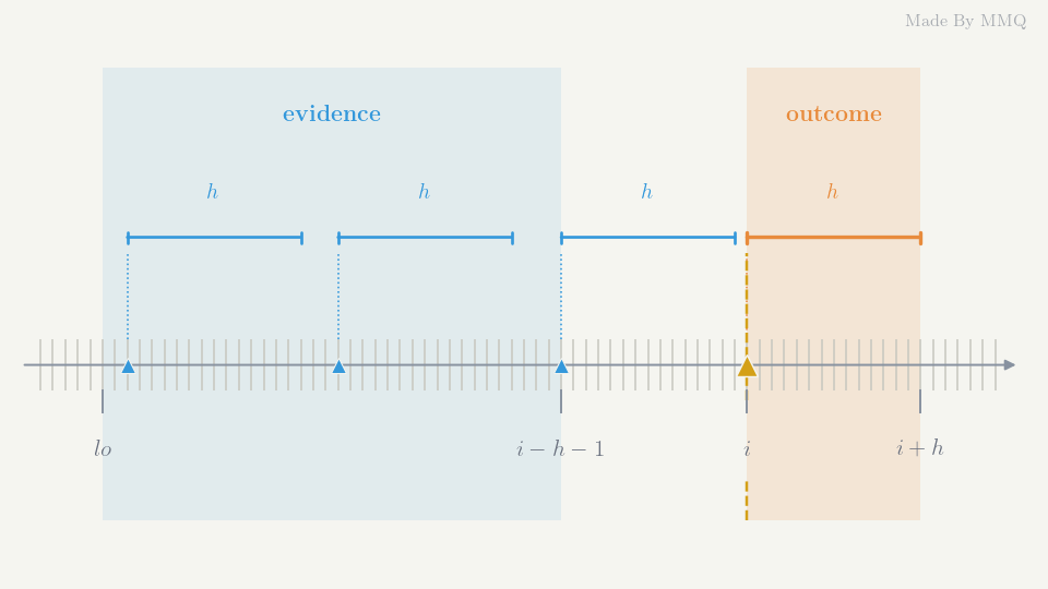
Fig. 4. The evidence window ends h bars before the firing so every return in it is observed; the outcome window begins at the firing and lies entirely in the future.
A null that respects the data
The null distribution comes from drawing the same number of bars out of the same window by stationary bootstrap and scoring them with the same multiset of directions. It is stationary rather than independent for one specific reason: forward windows of length h overlap, so consecutive entries share h-1 bars and are strongly autocorrelated. Resampling single bars destroys that dependence and produces a null far too narrow, which inflates every p-value's significance. Geometric blocks keep it.
//+------------------------------------------------------------------+
//| Draw n bar indices out of [lo,hi] by stationary bootstrap.       |
//|                                                                  |
//|  With probability 1/L a fresh uniform start is taken; otherwise  |
//|  the walk steps one bar forward and wraps at the top of the      |
//|  window. Block lengths are therefore geometric with mean L and   |
//|  the resampled series is stationary, which is what keeps the     |
//|  overlap structure of fwd[] intact.                              |
//+------------------------------------------------------------------+
void CPValueSource::Resample(const int lo,const int hi,const int n)
  {
   int len=hi-lo+1;
   double pnew=1.0/m_mean_block;
   int cur=m_rng.Integer(lo,hi);

   for(int k=0;k<n;k++)
     {
      if(k>0)
        {
         if(m_rng.Uniform()<pnew)
            cur=m_rng.Integer(lo,hi);
         else
            cur=lo+((cur-lo+1)%len);
        }
      m_draw[k]=cur;
     }
  }
The mean block length is therefore not a nuisance parameter. As a rule of thumb it should be at least the forward horizon, or the resampled series stops carrying the overlap the block bootstrap exists to preserve. Every run in this article uses a mean block of 20 against h = 10. That value satisfies the rule of thumb but was not tuned, and the p-values do depend on it, so treat 20 as a reasonable default rather than a proven optimum.
The floor that makes rejection impossible
The obvious way to turn the bootstrap into a p-value is to rank the observed statistic among the null draws. Doing exactly that produced the most instructive failure in this project.
A rank-based bootstrap p-value cannot be smaller than 1/(B+1), so B = 200 puts the floor at 0.005. Meanwhile LORD++ hands out a level of 0.0025 on the very first hypothesis and is down at 1e-4 by the twentieth if nothing has been discovered. The smallest p-value the source could physically produce was larger than the threshold it had to clear. Zero rejections were guaranteed by arithmetic, regardless of what the data said, and on a real symbol that looks exactly like a well-behaved conservative filter.
Raising B is not a practical rescue. Every bench here runs at B = 2000, which only moves the floor to 5.00e-04, still five times above the level LORD++ reaches after twenty quiet hypotheses. A floor of 1e-4 would cost B = 10000 replications for every hypothesis in the stream, and the level keeps falling faster than brute force can chase it.
The fix keeps the block-bootstrap null but reads its tail off a normal fitted to the draws, so the p-value is continuous and has no floor, at the cost of an explicit modelling assumption in the far tail where there are no draws to check it against. Both modes ship, along with the naive t-test, so the calibration bench can judge all three.
//+------------------------------------------------------------------+
//| How a firing is turned into a p-value.                           |
//|                                                                  |
//|  The choice is not a detail on a long stream. A rank-based       |
//|  bootstrap p-value cannot be smaller than 1/(B+1), and an online |
//|  procedure hands out levels far below that once the stream runs  |
//|  into the thousands -- LORD++ is already at 1e-4 by the twentieth|
//|  hypothesis if nothing has been discovered. A floor above the    |
//|  level makes rejection impossible no matter what the data says,  |
//|  which looks exactly like a well-behaved quiet gate and is not.  |
//|                                                                  |
//|  BOOT_NORMAL keeps the block-bootstrap null but reads the tail   |
//|  off a normal fitted to it, so the p-value is continuous and has |
//|  no floor. The cost is an explicit modelling assumption in the   |
//|  far tail, where there are no bootstrap draws to check it        |
//|  against. That is a real cost and the calibration bench is the   |
//|  only reason to believe it here.                                 |
//+------------------------------------------------------------------+
enum ENUM_FDR_PMODE
  {
   FDR_P_BOOTSTRAP,        // rank among the null draws; floor 1/(B+1)
   FDR_P_BOOT_NORMAL,      // normal fitted to the null draws; no floor
   FDR_P_TTEST             // naive t-test, the comparator that fails
  };
//+------------------------------------------------------------------+
//| Bootstrap p-value, one-sided in the direction of a real edge.    |
//|                                                                  |
//|  The (1+count)/(B+1) form is not cosmetic. Adding the observed   |
//|  statistic to its own null keeps the p-value valid at finite B:  |
//|  count/B can return exactly zero, and a p-value of zero is       |
//|  rejected by every procedure at every level, wealth or no        |
//|  wealth.                                                         |
//+------------------------------------------------------------------+
double CPValueSource::Evaluate(const double &fwd[],const int lo,const int hi,
                               const int &idx[],const double &dir[],const int n)
  {
   if(n<=0 || hi<=lo)
      return(1.0);

   if(m_mode==FDR_P_TTEST)
      return(TTest(fwd,idx,dir,n));

   double obs=Statistic(fwd,idx,dir,n);
   ArrayResize(m_draw,n);

   int ge=0;
   double sum=0.0,sumsq=0.0;
   for(int b=0;b<m_reps;b++)
     {
      Resample(lo,hi,n);
      double s=0.0;
      for(int k=0;k<n;k++)
         s+=dir[k]*fwd[m_draw[k]];
      s/=(double)n;
      m_null[b]=s;
      sum+=s;
      sumsq+=s*s;
      if(s>=obs)
         ge++;
     }

   if(m_mode==FDR_P_BOOTSTRAP)
      return((double)(1+ge)/(double)(m_reps+1));

//--- BOOT_NORMAL reads the bootstrap null's tail off a fitted normal,
//--- so it is continuous. The centre is estimated, not assumed zero.
   double mean=sum/(double)m_reps;
   double var =sumsq/(double)m_reps-mean*mean;
   if(var<FDR_EPS)
      return((obs>mean)?FDR_EPS:1.0);

   double z=(obs-mean)/MathSqrt(var);
   return(MathMin(1.0,MathMax(FDR_EPS,1.0-FdrNormalCdf(z))));
  }
The (1+count)/(B+1) form in the rank branch is also not cosmetic. Adding the observed statistic to its own null keeps the p-value valid at finite B: a plain count/B can return exactly zero, and a p-value of zero is rejected by every procedure at every level.
One detail in the normal branch: the centre is estimated from the draws, not assumed to be zero. A resampled null carries whatever drift the window had, and forcing its mean to zero would re-import the very bias the bootstrap exists to remove.
The glue walks the bars once and emits the candidate stream in time order, which is the order an online procedure must see. A firing without enough history is dropped rather than tested at a placeholder p-value, which would consume budget for a question nobody asked.
   for(int i=first;i<=last;i++)
     {
      int hi=FdrLastObservable(i,h);
      int lo=MathMax(first,i-m_lookback);
      if(hi-lo<m_min_hist*2)
         continue;

      for(int r=0;r<FDR_SIG_COUNT;r++)
        {
         int dir=bank.Direction(r,i);
         if(dir==0)
            continue;

         //--- the rule's own past firings inside the evidence window
         int n=0;
         ArrayResize(m_idx,0,256);
         ArrayResize(m_dir,0,256);
         for(int k=lo;k<=hi;k++)
           {
            int d=bank.Direction(r,k);
            if(d==0)
               continue;
            ArrayResize(m_idx,n+1,256);
            ArrayResize(m_dir,n+1,256);
            m_idx[n]=k;
            m_dir[n]=(double)d;
            n++;
           }

         if(n<m_min_hist)
            continue;

         src.SetMode(m_mode);
         double p=src.Evaluate(fwd,lo,hi,m_idx,m_dir,n);

         int m=ArraySize(out);
         ArrayResize(out,m+1,4096);
         out[m].bar =i;
         out[m].rule=r;
         out[m].dir =dir;
         out[m].p   =p;
         out[m].fwd =(double)dir*fwd[i];
         out[m].hist=n;
        }
     }
That excerpt is the body of the stream builder's main loop; the surrounding function handles allocation and the forward-return array.
Calibration Before the Market
On EURUSD there is no way to tell a procedure that controls FDR from one that does not, because nobody knows which rejections were true. Correctness has to be established where the answer is known, and CalibrationBench asks two questions in a fixed order, because the second is meaningless if the first fails.
Are the p-values valid?
A price series is generated with no edge by construction, the signal bank runs over it, and every firing is priced exactly as it would be live. Every one of those hypotheses is null, so the p-values must be well behaved.
The precise requirement is super-uniformity, meaning the probability that p is at or below x never exceeds x. It is weaker than uniformity, and the asymmetry is the point. A source returning too few small p-values is conservative: it costs power and nothing else. A source returning too many is manufacturing significance out of noise, and every guarantee downstream is void.
Our first attempt judged this with a two-sided Kolmogorov-Smirnov test, which cannot tell those two cases apart because it fails both: it condemned the block bootstrap, which runs below uniform over most of the range, alongside the genuinely broken comparator. The verdict has to be the one-sided statistic.
//+------------------------------------------------------------------+
//| One-sided KS statistic in the only direction that can break FDR  |
//| control: D+ = sup_x ( F_n(x) - x ).                              |
//|                                                                  |
//|  What the procedures require of a null p-value is SUPER-         |
//|  uniformity, P(p <= x) <= x, and not uniformity. A source        |
//|  returning too FEW small p-values is conservative: it costs      |
//|  power and nothing else, and every guarantee still holds. A      |
//|  source returning too MANY is manufacturing significance out of  |
//|  noise, and every guarantee downstream is void.                  |
//|                                                                  |
//|  A two-sided test cannot tell those apart -- it fails both. That |
//|  matters here, because a block bootstrap is conservative by      |
//|  construction, so judging it two-sided would condemn the correct |
//|  implementation alongside the broken one.                        |
//+------------------------------------------------------------------+
double FdrKsSuperUniform(double &p[],const int n)
  {
   if(n<2)
      return(1.0);

   ArraySort(p);
   double d=0.0;
   for(int i=0;i<n;i++)
      d=MathMax(d,(double)(i+1)/(double)n-p[i]);
   return(MathMax(d,0.0));
  }
Run over four null series of 6000 bars with B = 2000, giving 6148 null hypotheses, the t-test separates cleanly from the two bootstrap modes. Both parts of the bench use alpha 0.10, w0 0.05, lambda 0.50 and the LORD gamma sequence, seeded at 20260826.
| p-value mode | D+ | 5% critical | two-sided | P(p<0.01) | P(p<0.05) | smallest p | Verdict |
|---|---|---|---|---|---|---|---|
| bootstrap | 0.0101 | 0.0156 | 0.0339 | 0.0163 | 0.0395 | 5.00e-04 | Passes D+, excess below 0.01 |
| boot-normal | 0.0118 | 0.0156 | 0.0345 | 0.0184 | 0.0389 | 3.23e-13 | Passes D+, excess below 0.01 |
| t-test | 0.0828 | 0.0156 | 0.0828 | 0.0423 | 0.1074 | 5.43e-06 | Fails D+, invalid |
Read the two tail columns. Under a correct null, 5% of p-values should fall below 0.05: both bootstrap modes come in under that, while the t-test lands at more than double what it promises. Feed the t-test's p-values to LORD and the procedure faithfully controls a quantity that has nothing to do with the truth.
The 1% column is less comfortable, and it matters more. Below 0.01 the rank bootstrap returns 1.63% of its p-values and boot-normal 1.84%, so neither mode is conservative that deep in the tail, and the online levels live deeper still. D+ passes them because a Kolmogorov-Smirnov statistic measures the largest gap anywhere on the unit interval, and an excess confined to the far left is too small to move it. The bootstrap verdicts therefore mean "no gross failure", not "valid at the levels the procedures use".
The smallest-p column carries the other half of the story: the rank bootstrap bottoms out at exactly 1/(B+1), the floor discussed above, while boot-normal reaches 3.23e-13. That gap of nine orders of magnitude is the entire reason the second mode exists.

Fig. 5. Null p-value distributions in twenty bins. Both bootstrap modes sit at or below the uniform line in the first bin, though the excess below 0.01 is too fine for this binning to show; the t-test spikes to more than double it.
Do the procedures control FDR?
With the p-value source checked, a stream with a planted fraction of real effects goes to all five procedures. We run 2000 hypotheses per replication, 5% of them genuinely non-null, at an effect size of 3 standard deviations and a target FDR of 10%, averaged over 200 replications. These p-values are drawn exactly, so this part tests the procedures alone. It is also one scenario, and a strong one: real edges in trading rules are usually weaker and rarer, and power falls with them, so read the power column as a comparison between procedures, not as what to expect on a market.
| Procedure | Realised FDR | Power | Mean discoveries |
|---|---|---|---|
| uncorrected | 0.6691 | 0.9567 | 285.4 |
| bonferroni | 0.0013 | 0.0841 | 8.3 |
| lord3 | 0.0786 | 0.4021 | 43.4 |
| lord++ | 0.0266 | 0.3123 | 31.8 |
| saffron | 0.0242 | 0.3125 | 31.7 |
Two-thirds of what the uncorrected arm calls a discovery is noise, and it is the most confident of the five. Bonferroni is safe to the point of uselessness, buying its 0.13% realised FDR with 8% power. All three real procedures sit under the 10% target, with LORD3 closest to it and correspondingly the most powerful.
SAFFRON and LORD++ are indistinguishable here, which is worth stating plainly because the literature leads you to expect SAFFRON ahead. At lambda of 0.5 roughly half the null p-values are candidates, so the index shift and the (1 - lambda) scaling very nearly cancel for a gamma sequence of this shape. SAFFRON's advantage needs a smaller lambda or a denser alternative.
Where the Guarantee Breaks
Every result so far assumed independent p-values, which is what the proofs assume and what a trading stream is not. Publishing where a method breaks is worth more than publishing the method, so DependenceBench maps the failure envelope deliberately. The grid runs 100 replications per cell against the calibration bench's 200, so its independent row is this bench's own control and the two agree to within sampling error rather than exactly. No confidence intervals are tabled, and at 100 replications a cell close to 0.10 cannot be called either way with confidence; the verdicts below rest on the cells that are clearly over or clearly under. They also cover two dependence models from one generator, not every way a real stream can depend.
Two dependence regimes matter, and they do different amounts of damage. Block dependence models related instruments, or one rule seen through several timeframes, moving together; equicorrelated groups of twenty stand in for it. Burst dependence models one rule firing again a few bars later off an evidence window that barely moved. That is nearly the same hypothesis arriving repeatedly, and intuition says it should be the more corrosive of the two.
The measured answer contradicts that intuition, and reorders the three procedures.
| Regime | LORD3 FDR | LORD++ FDR | SAFFRON FDR | LORD3 throttled | SAFFRON throttled |
|---|---|---|---|---|---|
| independent | 0.0806 | 0.0257 | 0.0250 | 0.0806 | 0.0250 |
| block, rho 0.3 | 0.1252 | 0.0402 | 0.0570 | 0.0075 | 0.0075 |
| block, rho 0.6 | 0.1947 | 0.0554 | 0.1172 | 0.0100 | 0.0075 |
| block, rho 0.9 | 0.2396 | 0.0760 | 0.1542 | 0.0125 | 0.0050 |
| burst, length 3 | 0.0598 | 0.0224 | 0.0307 | 0.0369 | 0.0168 |
| burst, length 5 | 0.0577 | 0.0214 | 0.0325 | 0.0251 | 0.0105 |
| burst, length 10 | 0.0386 | 0.0228 | 0.0489 | 0.0179 | 0.0021 |
FDR is only half of the grid. The same run measures power, and every power figure quoted below comes from this table rather than from a log.
| Regime | LORD3 power | LORD++ power | SAFFRON power | LORD3 throttled |
|---|---|---|---|---|
| independent | 0.4056 | 0.3148 | 0.3180 | 0.4056 |
| block, rho 0.3 | 0.3720 | 0.2857 | 0.3011 | 0.2136 |
| block, rho 0.6 | 0.3669 | 0.2880 | 0.3088 | 0.2240 |
| block, rho 0.9 | 0.3401 | 0.2790 | 0.3080 | 0.2310 |
| burst, length 3 | 0.3244 | 0.2904 | 0.3027 | 0.3092 |
| burst, length 5 | 0.2736 | 0.2632 | 0.2751 | 0.2452 |
| burst, length 10 | 0.2310 | 0.2515 | 0.2736 | 0.2540 |
Three findings come out of the two grids, and only one was expected.
LORD++ is the robust one. It stays under the 10% target in every cell, reaching 0.0760 at the worst correlation tested. If you can only ship one procedure and you cannot characterise your dependence, this is the safest of the three on the evidence here.
LORD3 and SAFFRON both break under block dependence. LORD3 reaches 0.2396, nearly two and a half times its target, and SAFFRON 0.1542. Both violate the guarantee they advertise, and LORD3's extra power in the independent case is exactly what it cannot afford when the p-values correlate.
In this burst model, bursts hurt power, not FDR. Every procedure stays under target across all three burst lengths. At a within-burst correlation of 0.95 the repeats are so tightly bound that a null base draw usually produces repeats that are also large, so the burst rarely rejects at all. What it costs is discovery: LORD3 loses nearly half its power at burst length 10. That is a property of this generator at this correlation; weaker within-burst correlation was not tested and need not behave the same way.
The mitigation is a throttle: submit only the first hypothesis from a group within a gap, and drop the rest untested. It is a few lines.
//+------------------------------------------------------------------+
//| Keep only the first hypothesis of each group inside a gap.       |
//|                                                                  |
//|  A repeat arriving before the gap has elapsed is dropped without |
//|  being tested, which is the point: submitting it and accepting   |
//|  the answer would spend budget on a question already asked, and  |
//|  rejecting it a second time would double-count one discovery.    |
//+------------------------------------------------------------------+
int ApplyThrottle(const double &p[],const bool &truth[],const int &grp[],const int n,
                  const int gap,double &p_out[],bool &truth_out[])
  {
   int last[];
   int gmax=0;
   for(int i=0;i<n;i++)
      gmax=MathMax(gmax,grp[i]);
   ArrayResize(last,gmax+1);
   ArrayInitialize(last,-1000000);

   ArrayResize(p_out,n);
   ArrayResize(truth_out,n);

   int m=0;
   for(int i=0;i<n;i++)
     {
      int g=grp[i];
      if(i-last[g]<gap)
         continue;
      last[g]=i;
      p_out[m]    =p[i];
      truth_out[m]=truth[i];
      m++;
     }

   ArrayResize(p_out,m);
   ArrayResize(truth_out,m);
   return(m);
  }
The throttle restores control for all three procedures in every cell of the grid, driving LORD3 at rho 0.9 from 0.2396 down to 0.0125. Under block dependence it is not free: with a gap of 25 hypotheses a 2000-hypothesis stream is cut to 100, and LORD3's power in that cell falls with it. You buy back a guarantee you had lost by refusing to ask most of the questions.
Under bursts the trade is better, and in one cell it stops being a trade at all: at burst length 10 the throttle lifts LORD3's power while cutting its FDR. Dropping a repeat that was never going to reject costs no discoveries and saves the budget it would have spent, so the next genuinely new question is priced at a higher level. When your dependence is repetition rather than correlation, throttling is close to free, and repetition is the dependence a single-symbol signal stream mostly has.
Watching the Budget Drain
Run the full pipeline on 20000 bars of EURUSD H1, the window from 2023.06.08 to 2026.08.26, and the five rules produce 3428 tested hypotheses running from 2023.07.06 onward. The take-everything baseline over those firings has a mean signed forward return of -0.000040 and a hit rate of 0.490. There is no forward edge here, which makes the next table a test of something narrower than FDR control: whether what a gate accepts carries any more forward return than the stream it filters. On a market nobody labels the true and false discoveries, so no table in this section can confirm the guarantee itself.
Every number in this section and the next comes from one configuration, so it belongs on the page rather than in an input dialog. The Expert differs in two places only: a lighter bootstrap, because it recomputes on a live chart, and one procedure rather than five.
| Setting | StreamBench | FdrFilterEA |
|---|---|---|
| Forward horizon h | 10 bars | 10 bars |
| Bootstrap replications B | 2000 | 500 |
| Mean block length | 20 bars | 20 bars |
| Evidence window | 1500 bars | 1500 bars |
| Past firings needed to test | 25 | 25 |
| p-value mode | boot-normal | boot-normal |
| Procedure | all five | SAFFRON |
| Target FDR alpha | 0.10 | 0.10 |
| Initial wealth w0 | 0.05 | 0.05 |
| SAFFRON lambda | 0.50 | 0.50 |
| Gamma sequence | LORD | LORD |
| Starvation floor | 1e-4 | 1e-4 |
| Bootstrap seed | 20260826 | 20260826 |
All five procedures then see the identical stream, in the identical order, and the only thing that differs between the rows below is the level rule.
| Procedure | Accepted | Rate | Mean fwd, accepted | Mean fwd, blocked | Starved share |
|---|---|---|---|---|---|
| uncorrected | 382 | 0.1114 | 0.000018 | -0.000047 | 0.000 |
| bonferroni | 31 | 0.0090 | -0.000865 | -0.000033 | 0.989 |
| lord3 | 113 | 0.0330 | -0.000006 | -0.000041 | 0.575 |
| lord++ | 105 | 0.0306 | -0.000002 | -0.000041 | 0.333 |
| saffron | 107 | 0.0312 | 0.000003 | -0.000041 | 0.326 |
- The uncorrected arm is the scanner from the introduction, on real data. Its 382 discoveries carry a mean forward return under a fifth of a basis point over ten bars, comfortably inside the spread: 382 confident signals manufactured out of nothing.
- The gated procedures accept little, and what they accept does not trade. They accept about 3% of the stream and land near zero on the accepted side. That is not evidence that FDR was controlled. A rejection says the rule's past firings in its evidence window beat the bootstrap null, which can be true of the window without carrying into the next h bars. Had every hypothesis here been null in that sense, any rejection would be a false one, and control at 0.10 would allow a rejection on at most one run in ten, not a hundred of them. What the table shows is the gap between a statistical discovery and a tradable edge, which no FDR procedure closes.
- Bonferroni's accepted return is an outlier, not a result. It is computed over 31 accepts, far too few for a mean to carry information, and the accepted-side return of a procedure this quiet is mostly noise about noise.
- The last column is the practical story. It counts the share of hypotheses tested at a level below 1e-4. Boot-normal has no floor, so a p-value can still clear such a level, but only for a statistic about 3.7 standard deviations out; below it the gate is budget-limited in practice, if not in principle. Bonferroni spends 98.9% of the stream there, dead almost from the start, while LORD++ and SAFFRON spend a third of it.
The indicator
Wealth exhaustion is not a footnote, so it gets an instrument. AlphaWealth is a separate-window indicator plotting everything in log10, because the quantities live decades apart: over the run above, SAFFRON's admission level spans 0.0131 down to 1.33e-06 while the p-values feeding it reach 1e-12. On a linear axis only the wealth curve would be visible at all.
   double floor_v=SafeLog10(InpDeadLevel);
   int    first  =g_mon.FirstBar();

   for(int j=first;j<n;j++)
     {
      int i=g_begin+j;
      g_level[i] =SafeLog10(g_mon.Level(j));
      g_wealth[i]=SafeLog10(g_mon.Wealth(j));
      g_floor[i] =floor_v;

      double p=g_mon.PValue(j);
      if(p>=0.0)
         g_pval[i]=SafeLog10(p);

      double d=g_mon.Discovery(j);
      if(d>=0.0)
         g_disc[i]=SafeLog10(d);
     }
Read as one picture: the blue line is the bar the evidence has to clear, grey dots are the evidence that arrived, a dot below the line is a discovery marked in green, and the dashed red floor is where the level has sunk so low that only an extreme statistic can clear it. The blue line sinking toward that floor, and jumping back up on each green marker, is the mechanism made visible.
Cost is worth knowing before this goes on a live chart. Building the full 3428-hypothesis stream at B = 2000 takes about six seconds, paid once per replay rather than once per tick, and the indicator drops to B = 500 for the same reason. In steady state a new bar costs a single bootstrap against the evidence window.
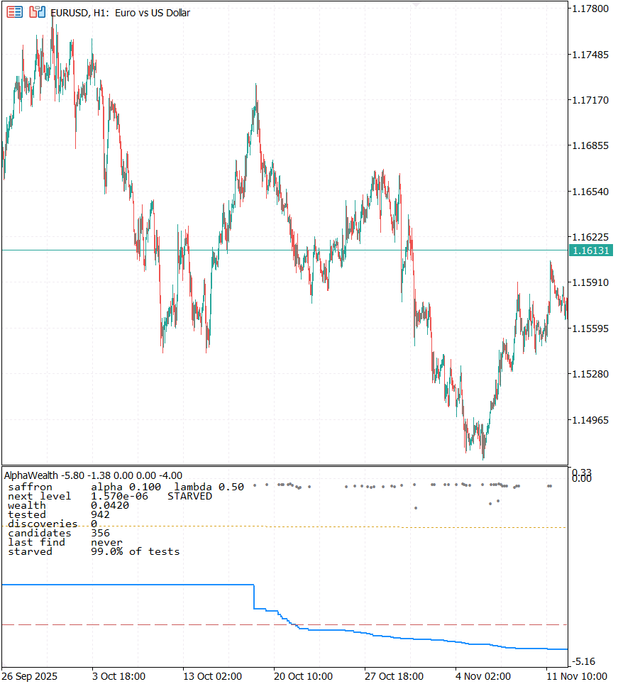
Fig. 6. The AlphaWealth subwindow on EURUSD H1. The admission threshold sinks toward the starvation floor between discoveries and jumps back on each green marker.
Driving this from an indicator forced one design change. An indicator is called on every bar and must not redo the past, because the procedures are order-dependent and a replay would silently produce different levels from the ones already drawn. CFdrMonitor therefore owns the procedure and the scan position together and exposes exactly two paths: a full replay from a clean procedure and a re-seeded bootstrap, or an append. Re-seeding is what makes a replay reproduce the run it replaces, since the bootstrap draws are the only randomness in the pipeline.
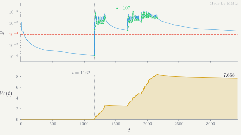
Fig. 7. The SAFFRON level and wealth trajectory over all 3428 hypotheses, plotted from the detail dump written by StreamBench.
The Gate Under Execution
Everything so far measures signals. FdrFilterEA asks whether any of it survives contact with spread and a position book. One Expert, one switch: GATE_OFF acts on every tested firing, GATE_ON only on those the procedure passed. Same rules, entries, exits and sizing, so the gate is the single difference between the arms.
Two design points are not free choices. The exit is a fixed hold of h bars, matching the horizon the p-value was computed over: holding for anything else would filter on one question and trade another. And the control arm takes every tested firing rather than every firing, since a firing without enough history was never priced and is not a hypothesis at all.
The demo runs SAFFRON, which needs a word given that the conclusion below recommends LORD++. On this stream the two are within two accepts of each other, and SAFFRON's free candidates are what make starvation legible on the panel: the level visibly stands still while candidates stream past and steps down only on large p-values. Where the recommendation bites is block dependence, which one symbol on one timeframe has far less of than a multi-symbol scanner.
//--- exits settle before entries. The counter resets ONLY on a
//--- confirmed close; a refused close must not report a hold of h.
   if(HasPosition())
     {
      g_hold++;
      if(g_hold>=InpHorizon && g_trade.PositionClose(_Symbol))
         g_hold=0;
     }

   int last=n-1;
   int tested=g_mon.SignalDir(last);
   if(tested==0)
      return;

   g_signals++;

//--- both arms record what the gate WOULD have passed, so the two
//--- logs compare directly.
   int acc=g_mon.AcceptedDir(last);
   if(acc!=0)
      g_accepted++;

   int dir=(InpGate==GATE_ON)?acc:tested;
   if(dir==0)
      return;

   if(HasPosition())
     {
      g_skipped++;
      return;
     }

   bool ok=(dir>0)?g_trade.Buy(InpLots,_Symbol):g_trade.Sell(InpLots,_Symbol);
   if(ok)
     {
      g_trades++;
      g_hold=0;
     }
   else
      g_failed++;
That exit block carries the second silent failure of the project. The first version reset the hold counter whether or not the close succeeded, and seventy order requests in that run were refused with "market closed". The table below counts refused entries only; the remainder were refused exits, and those did the damage, because an exit that failed while the counter reset anyway left the position open for longer than h bars while the Expert reported a hold of h. That broke the invariant the entire comparison rests on, and it flattered the gate: expected payoff read -0.904 against a true -1.493. Resetting only on a confirmed close fixes it, and a refused-entry counter makes the arithmetic reconcile.
Both arms on EURUSD H1, January 2024 to June 2026, SAFFRON at alpha 0.10, fixed 0.10 lots, and otherwise the configuration tabled in the previous section. That window is shorter than the one StreamBench measured, so the two sets of counts do not line up and neither is a check on the other.
| Measure | GATE_OFF (control) | GATE_ON (gated) |
|---|---|---|
| Signal bars | 2195 | 2195 |
| Passed by the gate | 116 | 116 |
| Skipped, book busy | 1232 | 22 |
| Refused by the server | 25 | 5 |
| Trades | 938 | 89 |
| Win rate | 0.4808 | 0.4831 |
| Expected payoff | -1.891 | -1.493 |
| Net profit | -1773.90 | -132.86 |
| Maximum drawdown | 19.08% | 2.95% |
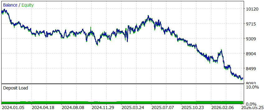
Fig. 8. Control arm. Every tested firing is acted on: 938 trades and a 19.08% drawdown.
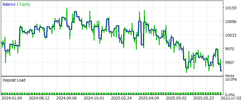
Fig. 9. Gated arm. The same rules behind the SAFFRON gate: 89 trades and a 2.95% drawdown.
Both arms lose money, and they should. The rules have no edge, as the previous section measured directly, and the Expert pays spread on top of that. No gate can rescue a system with nothing in it.
The gated arm makes 90% fewer trades, and most of its smaller loss and drawdown follows from that alone: fewer trades and less time in the market pay less spread and carry less risk. The per-trade figures do not separate the gate from that cut in exposure. Expected payoff differs by about 0.40 per trade, while a ten-bar EURUSD hold at 0.10 lots typically moves by tens of dollars, so on 89 trades that difference sits well inside its own noise; the win rates differ by far less than their standard error of about 0.053. This test cannot show that the gate picks better trades, only that it acts far less often.
Conclusion
We ported LORD3, LORD++ and SAFFRON into MQL5, built a causal p-value source for a live signal stream, and then spent most of the effort trying to break the result. What survived is worth more than the port.
- Validate the p-values before anything else, and validate them one-sided. FDR needs super-uniformity, not uniformity, and a two-sided test cannot tell a conservative source from a broken one. Then look past D+ to the far tail where the levels live: here both bootstrap modes passed D+ and still ran above nominal below 0.01. A source that is anti-conservative on pure noise voids the guarantee while leaving the arithmetic looking healthy, and a marginal check, however clean, does not establish the conditional validity the online proofs assume.
- Check your p-value resolution against your smallest level. A rank bootstrap floors at 1/(B+1). When that floor sits above the level the procedure assigns, zero rejections are arithmetically certain no matter what the data says, and it looks exactly like a well-behaved quiet gate. Raising B chases it only at a cost that grows with every quiet hypothesis: change the estimator, not the replication count.
- Of the three, prefer LORD++ when dependence is unknown. It held in every cell of the block and burst grid, while LORD3 and SAFFRON both broke the guarantee they advertise under block correlation. LORD3's extra power in the independent case is precisely what it cannot afford elsewhere. Two dependence models were tested, so this is the safest choice on the evidence here, not a guarantee against every kind of dependence.
- In the burst model tested, bursts cost power, not validity. Repeats generated at a within-burst correlation of 0.95 rarely reject at all; the damage was discoveries missed, not false ones made.
- Judge a quiet gate by its starved share. Silence can mean the market had nothing, or that the budget is so low that only an extreme statistic could get through. Only the starved fraction separates the two.
The outcome, and the reason to run any of this, is a bound you did not have before: provided the p-values are valid and the dependence is within what the bench covers, the expected share of acted-on signals that were noise stays below alpha. You cannot read that share off a live market, which is why the benches come first. Set alpha, run the calibration bench on your own rules, check the dependence table against how correlated your stream really is, then read the starved share on the panel. Treat the gate with suspicion when that share climbs past roughly one half, a practical warning level used in this article rather than one derived from the theory, and stop trusting it when the level sits below your p-value source's resolution floor. In that state the procedure is budget-limited rather than evidence-limited, and the honest response is to throttle the stream, not to lower alpha until something passes.
What this article does not do is make money, and the tester results say so directly. The five rules are a test bed for the methodology, chosen to be heterogeneous rather than profitable; point the same gate at rules that do carry an edge and the question becomes whether it still finds them once the budget competes.
The other direction is the scanner this article opened with. Its cells move together, and that is precisely the block dependence that broke LORD3 and SAFFRON above. The dependence table is the design document for that version: run LORD++, throttle correlated cells down to one submission per group per gap, and expect to buy the guarantee back with most of the questions.
Getting the Source Code via MQL5 Algo Forge
All source files are attached to this article below, but the full repository is also available on MQL5 Algo Forge, the community's Git-based platform for sharing and collaborating on trading projects.
| File name | Description |
|---|---|
| MQL5\Include\OnlineFDR\FdrCore.mqh | Shared vocabulary: procedures, p-value modes, gamma sequences, deterministic RNG and the normal CDF/quantile pair |
| MQL5\Include\OnlineFDR\FdrProcedures.mqh | LORD3, LORD++ and SAFFRON plus the uncorrected and online Bonferroni baselines, behind one interface |
| MQL5\Include\OnlineFDR\PValueSource.mqh | Stationary block bootstrap null with three p-value modes, and the forward-return helpers |
| MQL5\Include\OnlineFDR\SignalBank.mqh | Five heterogeneous close-only signal rules with incremental, bar-major storage |
| MQL5\Include\OnlineFDR\FdrStream.mqh | Batch glue turning a price series into a time-ordered stream of priced candidates |
| MQL5\Include\OnlineFDR\FdrSynthetic.mqh | Planted-truth hypothesis streams, three dependence regimes, null price series, FDP, power and the KS statistics |
| MQL5\Include\OnlineFDR\FdrMonitor.mqh | Incremental live engine driving one procedure bar by bar, with replay and append paths |
| MQL5\Scripts\OnlineFDR\CalibrationBench.mq5 | Bench: p-value validity on a null market, then FDR and power for all five procedures |
| MQL5\Scripts\OnlineFDR\DependenceBench.mq5 | Bench: the dependence failure envelope and the throttle mitigation |
| MQL5\Scripts\OnlineFDR\StreamBench.mq5 | Bench: the whole pipeline on real bars, with per-procedure and per-candidate dumps |
| MQL5\Indicators\OnlineFDR\AlphaWealth.mq5 | Separate-window indicator plotting the level, wealth, p-values, discoveries and starvation floor in log10, with a live readout |
| MQL5\Experts\OnlineFDR\FdrFilterEA.mq5 | Two-arm test bed running the same rules with the gate off and on |
Warning: All rights to these materials are reserved by MetaQuotes Ltd. Copying or reprinting of these materials in whole or in part is prohibited.
This article was written by a user of the site and reflects their personal views. MetaQuotes Ltd is not responsible for the accuracy of the information presented, nor for any consequences resulting from the use of the solutions, strategies or recommendations described.

 The MQL5 Standard Library Explorer (Part 17): Building a Reusable Portfolio Manager with CArrayObj
 Neural Networks in Trading: A Spiking-Semantic Approach to Spatiotemporal Identification (Key Components)
 Adaptive Trade Management in MQL5: Building a Broker-Aware, Deterministic, and Explainable Exit Engine
 Building a Prop Firm Compliance Monitor in MQL5 (Part 2): Daily Sessions and Restart-Safe Starting Balances

- Free trading apps
- Over 8,000 signals for copying
- Economic news for exploring financial markets
You agree to website policy and terms of use