Hierarchical Risk Parity: A Robust Portfolio Allocator and Expert Advisor

MetaTrader 5 — Trading systems | 6 August 2026, 12:06

142

Hammad Dilber

Introduction: When the Optimizer Turns on You

Every trader who runs more than one instrument eventually hits the same quiet question. You have a fixed amount of capital and a handful of markets you want exposure to, say EURUSD, GBPUSD, USDJPY, gold, and a stock index. How much of that capital should each one receive? Split it equally and you ignore that gold can swing several times more violently than a currency pair on any given day. Guess by feel and you are one rough week away from wishing you had a rule. The allocation decision is not glamorous, but it quietly shapes how smooth or how brutal your equity curve turns out to be.

The classic answer is mean-variance optimization, the framework Harry Markowitz published in 1952. You give it the covariance matrix of the instruments' returns, and it hands back the exact weights that minimize the portfolio's variance. On paper it is elegant and complete. On real market data it is also, more often than anyone would like, treacherous.

The trouble hides inside a single operation. To find its optimal weights, mean-variance optimization has to invert the covariance matrix. Inversion is well behaved only when the instruments are reasonably distinct from one another, and in trading they rarely are. EURUSD and GBPUSD move together most of the time. Two stock indices are often the same trade wearing different names. When instruments are that similar, the covariance matrix becomes close to singular, and inverting it starts to resemble dividing by a number that is almost zero. Tiny, meaningless wiggles in the estimated correlations get amplified into large, confident-looking positions.

The symptom is easy to recognize once you have seen it. The optimizer decides the best portfolio is a heavy long in one instrument financed by an equally heavy short in a near-identical one, leveraged well beyond the capital you actually hold. Shift the estimation window by a few bars and the whole prescription can flip. These weights are not wrong in the arithmetic sense. They really are the minimum-variance solution for the numbers you fed in. They are simply built on noise, and noise does not repeat.

Hierarchical Risk Parity, introduced by Marcos Lopez de Prado in 2016, takes a different route to the same destination. It never inverts the covariance matrix, so it never sets off the instability in the first place. Instead of treating all the instruments as one pool to optimize over, it first uncovers the structure already sitting in the data: which instruments behave alike, and how they group into families. It arranges them into a tree by similarity, then pours capital down that tree, splitting at each branch in proportion to risk.

This article implements the method as a single MQL5 class, CHRPAllocator, and explains it step by step. Each stage is verified against an independent Python reference. Real-data examples show why HRP avoids the leverage blow-up seen in Markowitz. The allocator is also packaged into a rebalancing Expert Advisor for any basket. HRP is a risk allocator, not a return forecaster, and the article keeps that distinction honest throughout.

What the Allocator Produces

It helps to see the finished product before taking it apart. The object the class produces is nothing exotic: a list of weights, one per instrument, all positive and adding up to one hundred percent of your capital. Hand the allocator 250 hourly bars for a five-instrument basket and it returns something you could act on right away.

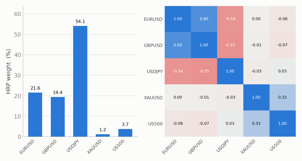
Left: bar chart of five positive HRP weights summing to one. Right: correlation heatmap of the five instruments

Fig. 1. HRP weights for a five-instrument basket (left) and the pairwise correlation the allocator reads (right); EURUSD and GBPUSD are strongly correlated, so they share one risk budget

The bar chart on the left is the output, a clean long-only allocation with no shorts and no leverage. The heatmap on the right is the raw material the allocator reads, the pairwise correlation of the five instruments. The two are linked. EURUSD and GBPUSD are strongly correlated, which the heatmap shows as a bright cell where they cross. HRP notices this and treats the pair as a single family that shares one risk budget, rather than naively handing each a full slice and doubling up on the same bet. That instinct, to recognize redundancy and refuse to over-commit to it, is the whole point of the method.

That is what the class delivers. The sections that follow explain how it gets from the heatmap on the right to the bars on the left, and why those bars stay sane where the classic optimizer's do not.

The Three Ideas Behind HRP

Underneath the name, HRP is just three ideas applied one after another. None of them is complicated on its own, and together they replace the fragile matrix inversion with something more robust.

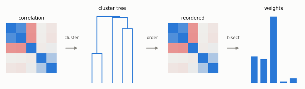
Flow diagram: correlation matrix to cluster tree to reordered matrix to weights

Fig. 2. The three stages of HRP: the correlation matrix becomes a cluster tree, the tree fixes an ordering that block-diagonalizes the matrix, and recursive bisection turns that order into weights

The first idea is tree clustering. We turn the correlation matrix into a distance, so that instruments which behave alike sit close together and instruments which behave differently sit far apart. Then we group them into a binary tree, where the most similar pairs merge first and end up as neighbors deep inside the tree. This is the step that discovers structure, and it is what lets us avoid inverting anything at all.

The second idea is quasi-diagonalization. The tree tells us which instruments belong together, but it does not by itself hand us an order. Walking the tree from top to bottom produces a sequence in which similar instruments end up side by side. Reorder the correlation matrix by that sequence and the large values slide toward the diagonal and gather into neat blocks. The matrix becomes almost diagonal, which is where the awkward name comes from, and those blocks are the families we want to budget across.

The third idea is recursive bisection. Take the ordered list, cut it in half, and compare the risk of the two halves. Give more capital to the calmer half and less to the wilder one. Then cut each half in half again and repeat, working down until every piece is a single instrument. Capital trickles down the tree, and at every fork it leans toward the safer branch.

The class implements these three ideas as five methods, because the first idea needs two preparation steps before it can run. The full pipeline is: compute returns, build the covariance and correlation matrices, grow the cluster tree, read off the ordering, and run the bisection. The sections below take them in that order.

From Prices to Correlation

The class stores its intermediate results as native MQL5 matrices and a few plain arrays. Here is the full interface.

//+------------------------------------------------------------------+
//| CHRPAllocator - Hierarchical Risk Parity allocator               |
//|                                                                  |
//|  Pipeline (Lopez de Prado, 2016):                                |
//|    1. CalculateReturns()   - price bars  -> simple returns       |
//|    2. BuildCovCorr()       - returns     -> cov + corr matrices  |
//|    3. HierarchicalCluster()- corr        -> AHC linkage tree     |
//|    4. QuasiDiagonal()      - tree       -> reordered leaf order  |
//|    5. RecursiveBisection() - order+cov   -> final weights[]      |
//|                                                                  |
//|  No matrix inversion anywhere: robust to correlated assets.      |
//+------------------------------------------------------------------+
class CHRPAllocator
  {
private:
   int               m_nAssets;      // number of symbols in the basket
   int               m_nObs;         // number of return observations per asset

   matrix            m_returns;      // [m_nObs x m_nAssets] simple returns
   matrix            m_cov;          // [m_nAssets x m_nAssets] covariance
   matrix            m_corr;         // [m_nAssets x m_nAssets] correlation

   int               m_order[];      // quasi-diagonal leaf ordering (len m_nAssets)
   double            m_weights[];    // final HRP weights (len m_nAssets)

   //--- stage 3 output: single-linkage merge tree (m_nAssets-1 merges).
   //    Merge i forms cluster (m_nAssets + i); children are original
   //    leaves (< m_nAssets) or earlier clusters (>= m_nAssets).
   matrix            m_dist;         // correlation distance sqrt(0.5*(1-corr))
   int               m_linkA[];      // first child of merge i   (Z[i,0])
   int               m_linkB[];      // second child of merge i  (Z[i,1])
   double            m_mergedist[];  // distance at which merge i happened

   //--- recursive leaf expansion for quasi-diagonalization
   void              ExpandNode(int node, int &out[], int &cnt) const;

   //--- inverse-variance-weighted variance of the cluster m_order[s..e-1]
   double            ClusterVar(int s, int e) const;

public:
                     CHRPAllocator();
                    ~CHRPAllocator() {}

   //--- full pipeline: closes[nBars][nAssets] price panel -> weights[]
   bool              Solve(const matrix &closes);

   //--- individual stages (exposed for per-stage verification) ------
   bool              CalculateReturns(const matrix &closes);
   bool              BuildCovCorr();
   bool              HierarchicalCluster();
   bool              QuasiDiagonal();
   bool              RecursiveBisection();

   //--- accessors ---------------------------------------------------
   int               Size()          const { return m_nAssets; }
   int               Obs()           const { return m_nObs; }
   void              GetWeights(double &out[]) const { ArrayCopy(out, m_weights); }
   void              GetOrder(int &out[])      const { ArrayCopy(out, m_order); }
   matrix            Returns()        const { return m_returns; }
   matrix            Corr()           const { return m_corr; }
   matrix            Cov()            const { return m_cov; }
   matrix            Dist()           const { return m_dist; }
   void              GetLinkage(int &a[], int &b[], double &d[]) const
                       { ArrayCopy(a, m_linkA); ArrayCopy(b, m_linkB); ArrayCopy(d, m_mergedist); }
  };

Each of the five stages is its own public method, rather than being buried inside a single call. The reason is verification. Because every stage can be run and inspected on its own, we can export its output and compare it against an independent reference, which is exactly what we do later. The Solve method is a thin driver that runs the five stages in order.

The first stage converts prices into returns. Its input is a price panel with bars in rows and instruments in columns, arranged oldest bar first. Its output is a matrix of one-step returns.

//+------------------------------------------------------------------+
//| Stage 1 - simple returns from a [nBars x nAssets] close panel    |
//|   r[t][a] = closes[t+1][a] / closes[t][a] - 1                    |
//|   rows run oldest -> newest (chronological), so the numpy        |
//|   cross-check on the same closes reproduces these 1:1.           |
//+------------------------------------------------------------------+
bool CHRPAllocator::CalculateReturns(const matrix &closes)
  {
   int nBars = (int)closes.Rows();
   m_nAssets = (int)closes.Cols();
   if(nBars < 3 || m_nAssets < 2)
     {
      Print("CHRPAllocator::CalculateReturns - need >=3 bars and >=2 assets");
      return false;
     }
   m_nObs = nBars - 1;
   m_returns.Init(m_nObs, m_nAssets);
   for(int t = 0; t < m_nObs; t++)
      for(int a = 0; a < m_nAssets; a++)
        {
         double p0 = closes[t][a];
         double p1 = closes[t + 1][a];
         if(p0 <= 0.0) return false;
         m_returns[t][a] = p1 / p0 - 1.0;
        }
   return true;
  }

These are simple returns, the next price divided by the current price minus one. There are two common conventions, and they are not interchangeable. Simple returns are what Lopez de Prado uses in the original HRP code, and they keep the later cross-check clean, so that is the convention here. With a panel of N bars we get N-1 return observations. The guard at the top rejects a panel that is too short or holds only a single instrument, since one instrument has nothing to be allocated against.

The second stage turns those returns into two matrices, both needed downstream for different reasons. The correlation matrix drives the clustering, because clustering is about which instruments move together. The covariance matrix drives the risk budgeting, because budgeting is about how large those moves actually are.

//+------------------------------------------------------------------+
//| Stage 2 - sample covariance + Pearson correlation of returns     |
//|   cov uses ddof = 1 (denominator nObs-1) to match numpy cov      |
//+------------------------------------------------------------------+
bool CHRPAllocator::BuildCovCorr()
  {
   //--- column means
   vector mean(m_nAssets);
   for(int a = 0; a < m_nAssets; a++)
     {
      double s = 0.0;
      for(int t = 0; t < m_nObs; t++) s += m_returns[t][a];
      mean[a] = s / m_nObs;
     }
   //--- covariance (symmetric), denominator nObs-1
   m_cov.Init(m_nAssets, m_nAssets);
   double denom = (double)(m_nObs - 1);
   for(int i = 0; i < m_nAssets; i++)
      for(int j = i; j < m_nAssets; j++)
        {
         double s = 0.0;
         for(int t = 0; t < m_nObs; t++)
           s += (m_returns[t][i] - mean[i]) * (m_returns[t][j] - mean[j]);
         double c = s / denom;
         m_cov[i][j] = c;
         m_cov[j][i] = c;
        }
   //--- correlation from covariance
   m_corr.Init(m_nAssets, m_nAssets);
   for(int i = 0; i < m_nAssets; i++)
      for(int j = i; j < m_nAssets; j++)
        {
         double r = m_cov[i][j] / MathSqrt(m_cov[i][i] * m_cov[j][j]);
         m_corr[i][j] = r;
         m_corr[j][i] = r;
        }
   return true;
  }

The covariance uses the sample estimator with the standard denominator of the number of observations minus one, which matches what numpy produces by default and keeps the later comparison exact. The correlation is the ordinary Pearson form: each covariance entry divided by the product of the two standard deviations. Both matrices are symmetric, so each inner loop starts at the diagonal and writes both mirror positions at once. The full source also guards against an instrument whose variance came out at zero, which would make its correlation undefined; that check lives in the file but is left out of the listing here to keep the calculation clear.

At the end of this stage we hold the correlation matrix, which is the heatmap shown earlier. The next stage is the first genuinely HRP-specific step, and it reads that matrix.

Building the Cluster Tree

A subtle problem stands between the correlation matrix and the tree. Correlation is not a distance, and clustering algorithms expect a distance. Two instruments with a correlation of one behave identically, so the distance between them should be zero. Two with a correlation of minus one move in perfect opposition, which is still a strong and usable relationship, so they should not be infinitely far apart either. The standard HRP transform captures both intuitions in one formula.

d(i,j) = sqrt( 0.5 * (1 - corr(i,j)) )

A correlation of one maps to a distance of zero, a correlation of zero maps to about 0.707, and a correlation of minus one maps to a distance of one. The result is a proper metric, which is the property the clustering algorithm relies on. With the distance matrix built, we hand the actual clustering to ALGLIB, which ships with the standard MQL5 installation and saves us from writing an agglomerative clusterer by hand.

//+------------------------------------------------------------------+
//| Stage 3 - single-linkage AHC on distance d=sqrt(0.5*(1-corr))    |
//|   Correlation is turned into a proper metric, then ALGLIB's      |
//|   agglomerative clusterer builds the merge tree.                 |
//+------------------------------------------------------------------+
bool CHRPAllocator::HierarchicalCluster()
  {
   //--- correlation distance matrix (0 diagonal, symmetric)
   m_dist.Init(m_nAssets, m_nAssets);
   CMatrixDouble dmat;
   dmat.Resize(m_nAssets, m_nAssets);
   for(int i = 0; i < m_nAssets; i++)
      for(int j = 0; j < m_nAssets; j++)
        {
         double d = (i == j ? 0.0 : MathSqrt(0.5 * (1.0 - m_corr[i][j])));
         m_dist[i][j] = d;
         dmat.Set(i, j, d);
        }
   //--- ALGLIB agglomerative clustering, single linkage
   CClusterizerState state;
   CAHCReport        rep;
   CClustering::ClusterizerCreate(state);
   CClustering::ClusterizerSetDistances(state, dmat, m_nAssets, false);
   CClustering::ClusterizerSetAHCAlgo(state, 1);  // 1 = single linkage
   CClustering::ClusterizerRunAHC(state, rep);
   if(rep.m_terminationtype <= 0) return false;
   //--- copy the merge tree (Z) and merge distances
   int nMerge = m_nAssets - 1;
   ArrayResize(m_linkA, nMerge);
   ArrayResize(m_linkB, nMerge);
   for(int i = 0; i < nMerge; i++)
     {
      m_linkA[i] = rep.m_z.Get(i, 0);
      m_linkB[i] = rep.m_z.Get(i, 1);
     }
   return true;
  }

We build the distance matrix into two places at once. One is a native matrix kept for the verification export. The other is the ALGLIB CMatrixDouble the clusterizer consumes. Four calls then do the work: create the state, give it the distances, choose the linkage rule, and run. The linkage rule decides how the distance between two whole clusters is measured, and Lopez de Prado's original HRP uses single linkage, which defines that distance as the gap between the two nearest members. We select it by passing algorithm code one.

What comes back is the merge tree, which ALGLIB returns as a Z matrix with one row per merge. The numbering matters for the next stage. The original instruments are numbered zero through N-1. The first merge creates a new cluster numbered N, the second creates one numbered N+1, and so on. Each row names the two children joined at that step, and a child is either an original instrument or a cluster from an earlier merge. We copy the two child columns into plain arrays. This tree is what a dendrogram draws.

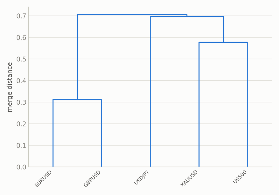
Dendrogram of five instruments; EURUSD and GBPUSD merge first at a low height, gold and the index join later

Fig. 3. Single-linkage cluster tree of the basket; EURUSD and GBPUSD merge first at a small distance, gold and the index form a second pair, and USDJPY joins them higher up

The dendrogram turns the tree into something you can read at a glance. Instruments that behave alike join low, at a small merge distance, and the height at which two branches meet is the distance between their clusters. Reading it from the bottom up is like watching the market sort its own instruments into families, without anyone telling it which are currencies and which are metals. The structure is discovered from the returns themselves, not imposed by hand.

Quasi-Diagonalization

The tree knows which instruments belong together, but it does not give us a single ordered list, and the risk budgeting works on an ordered list. Quasi-diagonalization produces one by walking the tree from its root down to the leaves. At every internal node it descends into both children before moving on, so the leaves come out in an order where tree-neighbors are list-neighbors.

A short recursive helper performs the walk. Given a node, if the node is an original instrument then it is a leaf, so we record it and return. Otherwise it is a cluster, and we recurse into its two children.

//+------------------------------------------------------------------+
//| Depth-first expansion of a tree node into its original leaves    |
//+------------------------------------------------------------------+
void CHRPAllocator::ExpandNode(int node, int &out[], int &cnt) const
  {
   if(node < m_nAssets)           // original asset leaf
     { out[cnt++] = node; return; }
   int j = node - m_nAssets;       // internal cluster formed at merge j
   ExpandNode(m_linkA[j], out, cnt);
   ExpandNode(m_linkB[j], out, cnt);
  }

//+------------------------------------------------------------------+
//| Stage 4 - quasi-diagonalization: walk the tree from the root     |
//|   down to leaves, producing the ordering that places similar     |
//|   assets adjacent (Lopez de Prado's getQuasiDiag).               |
//+------------------------------------------------------------------+
bool CHRPAllocator::QuasiDiagonal()
  {
   int nMerge = m_nAssets - 1;
   ArrayResize(m_order, m_nAssets);
   int cnt  = 0;
   int root = m_nAssets + (nMerge - 1);  // last merge = top of the tree
   ExpandNode(root, m_order, cnt);
   return (cnt == m_nAssets);
  }

The starting point is the root, which is always the last merge the algorithm performed, because that final join unites everything into a single cluster. Expanding it fills the order array with all N instruments. The check at the end confirms every leaf was reached exactly once, a cheap guard against a malformed tree. The recursion depth can never exceed the number of instruments, and a realistic basket has a handful, so a plain recursive walk is both the clearest and the safest way to write this.

The reward for the ordering is easiest to appreciate visually. Reorder the rows and columns of the correlation matrix by the new sequence and the strong values migrate off the periphery and gather near the diagonal.

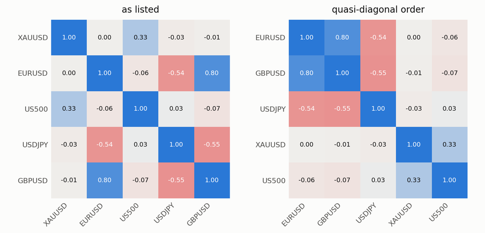
Two heatmaps side by side; after reordering the strong correlations form blocks along the diagonal

Fig. 4. The same correlation matrix listed in an arbitrary order (left) and in the quasi-diagonal order (right), where the strong values gather into blocks along the diagonal

The left panel is the raw correlation matrix in whatever order the instruments were listed. The right panel is the same matrix after quasi-diagonalization. The strong correlations, scattered before, now consolidate into blocks running down the diagonal. Each block is a family of related instruments, and those families are the groups the final stage will budget capital across.

Recursive Bisection

This stage assigns the capital, and it is the heart of the method. It operates entirely on the ordered list. Cut the list into two halves, measure the risk of each half, and give the calmer half a larger share. Then cut each half in two and repeat, until every piece is a single instrument holding its final weight.

To compare two halves we need a way to boil the risk of a group down to a single number. The cluster-variance helper does that. For a given cluster it first forms an inverse-variance portfolio inside the group, meaning each member is weighted by one over its own variance and those weights are normalized. It then runs that internal weight vector through the covariance matrix to get the variance of the cluster as a whole.

//+------------------------------------------------------------------+
//| Inverse-variance-portfolio variance of cluster m_order[s..e-1]   |
//|   w_i = (1/var_i) / sum(1/var), cVar = w' * cov * w              |
//+------------------------------------------------------------------+
double CHRPAllocator::ClusterVar(int s, int e) const
  {
   int len = e - s;
   double ivp[];
   ArrayResize(ivp, len);
   double sum = 0.0;
   for(int k = 0; k < len; k++)
     {
      int idx = m_order[s + k];
      ivp[k]  = 1.0 / m_cov[idx][idx];
      sum    += ivp[k];
     }
   for(int k = 0; k < len; k++) ivp[k] /= sum;
   double cVar = 0.0;
   for(int a = 0; a < len; a++)
      for(int b = 0; b < len; b++)
        cVar += ivp[a] * m_cov[m_order[s + a]][m_order[s + b]] * ivp[b];
   return cVar;
  }

The inverse-variance weighting inside a cluster is a sensible default: within a group, lean toward the calmer members. The double loop is the standard quadratic form that turns a weight vector and a covariance matrix into a single variance figure. Notice what is absent. There is no matrix inversion here, only direct reads of the covariance entries and the diagonal variances. This is exactly where HRP sidesteps the trap that catches mean-variance optimization.

The bisection keeps a working list of clusters, each described by a start and an end index into the ordered array. It begins with the entire list as one cluster and every instrument holding a provisional weight of one.

//+------------------------------------------------------------------+
//| Stage 5 - recursive bisection (Lopez de Prado getRecBipart).     |
//|   Split the quasi-diagonal order in half repeatedly; at each     |
//|   split give the two sides weight in inverse proportion to their |
//|   cluster variance, so riskier clusters receive less capital.    |
//+------------------------------------------------------------------+
bool CHRPAllocator::RecursiveBisection()
  {
   ArrayResize(m_weights, m_nAssets);
   ArrayInitialize(m_weights, 1.0);
   //--- clusters as [start,end) slices into m_order
   int cs[], ce[];
   ArrayResize(cs, 1); ArrayResize(ce, 1);
   cs[0] = 0; ce[0] = m_nAssets;
   while(ArraySize(cs) > 0)
     {
      //--- bisect every cluster of length > 1 into two halves
      int ns[], ne[];
      int cnt = 0;
      for(int c = 0; c < ArraySize(cs); c++)
        {
         int s = cs[c], e = ce[c];
         if(e - s <= 1) continue;
         int mid = s + (e - s) / 2;
         ArrayResize(ns, cnt + 2); ArrayResize(ne, cnt + 2);
         ns[cnt] = s;   ne[cnt] = mid;
         ns[cnt+1] = mid; ne[cnt+1] = e;
         cnt += 2;
        }
      //--- allocate across each (left,right) pair by cluster variance
      for(int i = 0; i < cnt; i += 2)
        {
         double v0 = ClusterVar(ns[i],   ne[i]);
         double v1 = ClusterVar(ns[i+1], ne[i+1]);
         double alpha = 1.0 - v0 / (v0 + v1);
         for(int k = ns[i];   k < ne[i];   k++) m_weights[m_order[k]] *= alpha;
         for(int k = ns[i+1]; k < ne[i+1]; k++) m_weights[m_order[k]] *= (1.0 - alpha);
        }
      ArrayCopy(cs, ns); ArrayCopy(ce, ne);
      ArrayResize(cs, cnt); ArrayResize(ce, cnt);
     }
   return true;
  }

Each pass through the outer loop slices every cluster that still holds more than one instrument into a left half and a right half. For each pair we compute the two cluster variances and derive a single split factor.

alpha = 1 - v0 / (v0 + v1)

The left half is multiplied by alpha and the right half by one minus alpha. If the left cluster is the riskier of the two, its variance v0 is large, alpha comes out small, and the left side receives the smaller share. That is risk parity compressed into a single line: at every fork, capital drifts toward the calmer branch. Because each instrument's final weight is the running product of the split factors along its path, and because the two factors at any split add up to one, the weights automatically sum to one at the end. There is no separate normalization step to remember.

The loop stops when no cluster can be split further, which is when every surviving slice holds one instrument. At that moment the weights array holds the final allocation.

Verifying the Pipeline

The five stages are tied together by a single driver, so a caller never runs them by hand.

//+------------------------------------------------------------------+
//| Full pipeline driver                                             |
//+------------------------------------------------------------------+
bool CHRPAllocator::Solve(const matrix &closes)
  {
   if(!CalculateReturns(closes)) return false;
   if(!BuildCovCorr())           return false;
   if(!HierarchicalCluster())    return false;
   if(!QuasiDiagonal())          return false;
   if(!RecursiveBisection())     return false;
   return true;
  }

Pass in a price panel, get back a success flag, then read out the weights. That is the entire public interface a strategy needs. Because the pipeline has multiple stages, each stage was verified against an independent Python implementation before using it with real capital. A companion MQL5 script runs the allocator on a real basket and exports each intermediate result to CSV: the closes, the covariance and correlation matrices, the distance matrix, the cluster tree, the ordering, and the final weights. A Python script reloads those same closes and recomputes each stage from scratch with numpy and scipy.

The comparison is performed stage by stage. If only the final weights were compared, any mismatch would not identify which of the five stages caused the error. Checking each stage in isolation points any discrepancy straight at its source. In practice the agreement is essentially exact. The covariance and correlation match numpy to within about 10^-14. The single-linkage merge heights match the scipy clustering exactly. The quasi-diagonal ordering, replayed from the exported tree, matches the Python walk element for element. And the final weights match the canonical Lopez de Prado recursion to within about 10^-16, the floor of double-precision arithmetic.

One point about the verification deserves a plain statement. The export script loads each instrument by bar index rather than by aligning timestamps across instruments. That is harmless here, because the Python side reads the exact same exported panel, so both computations see identical inputs. Timestamp alignment only matters when the allocator runs live on instruments with different trading hours, and the Expert Advisor later in this article handles that case properly.

Why HRP and Not Markowitz

A verified allocator is not the same as a useful one. The natural benchmark is the method HRP was designed to replace, Markowitz minimum-variance. The minimum-variance weights have a closed form, and writing it out shows the exact operation HRP avoids.

//+------------------------------------------------------------------+
//| Markowitz minimum-variance weights: w = Cov^-1 1 / (1' Cov^-1 1) |
//+------------------------------------------------------------------+
bool MinVarWeights(const matrix &cov, double &w[])
  {
   int n = (int)cov.Rows();
   matrix inv = cov.Inv();
   if(inv.Rows() != n) return false;   // singular
   ArrayResize(w, n);
   double sum = 0.0;
   for(int i = 0; i < n; i++)
     {
      double raw = 0.0;
      for(int j = 0; j < n; j++) raw += inv[i][j];
      w[i] = raw; sum += raw;
     }
   if(MathAbs(sum) < 1e-300) return false;
   for(int i = 0; i < n; i++) w[i] /= sum;
   return true;
  }

The whole method hinges on the single call to Inv. On a calm five-instrument basket that inversion is harmless, and the two methods produce nearly identical, sensible weights. The interesting behavior appears when the instruments become more correlated or more numerous, because that is when the covariance matrix becomes hard to invert. To stress it, we run both methods on a 21-instrument basket of currencies, crosses, metals, and indices, estimated from only 30 bars, so the matrix is nearly singular.

The contrast is stark. Running both allocators on that basket, side by side, gives the following.

Metric (21 symbol)	HRP	Markowitz	Equal-Weight (1/N)
Gross exposure	100%	331%	100%
Short positions	0	8	0
Smallest weight	+0.10%	-43.6%	+4.76%
Largest weight	+17.5%	+58.8%	+4.76%

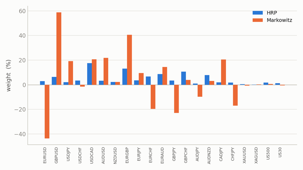
Grouped bar chart; HRP bars are all positive and modest, Markowitz bars swing from large negative to large positive

Fig. 5. HRP versus Markowitz weights on a 21-instrument basket estimated from only 30 bars; Markowitz swings from a 44 percent short to a 59 percent long, while HRP stays modest and long-only

The third column is the naive baseline: a plain equal-weight book that gives every instrument the same +4.76% share, which is 100% divided by the 21 instruments. It never inverts anything either, so it stays long-only and fully invested by construction. Markowitz responds to the near-singular matrix by building a heavily leveraged long-short book, with a 43.6% short in one instrument and gross exposure over three times the account. HRP on the same data stays long-only, caps its largest holding near 17.5%, and keeps gross exposure at exactly one hundred percent. HRP lands in the same safe envelope as equal-weight, long-only and unlevered, but it spreads capital by the correlation structure instead of blindly, so it is the robust baseline made risk-aware rather than the fragile optimizer. This is the failure mode from the introduction, made concrete. HRP does not produce it, because it never inverts the matrix.

A Rebalancing Expert Advisor

Turning the allocator into a live trader is mostly plumbing, with one genuine engineering problem. A basket that mixes a currency pair with a stock index mixes instruments that trade on different schedules, so their bars do not line up one to one. Feeding misaligned bars into the covariance calculation quietly corrupts it. A helper named AlignedCloses, whose full listing is in the attached Expert Advisor, solves this by building a price panel only from the timestamps that every instrument in the basket shares, so every row of the panel is a moment all instruments were trading.

With aligned prices in hand, the rebalance is short. It solves for the HRP weights, converts each weight into a target position size, closes whatever the Expert Advisor currently holds, and opens the fresh targets.

//+------------------------------------------------------------------+
//| Compute HRP weights and rebuild the basket at target sizes.      |
//+------------------------------------------------------------------+
void Rebalance()
  {
   Print("[HRP-EA] rebalance triggered @ ", TimeToString(TimeCurrent()));
   matrix closes;
   if(!AlignedCloses(InpLookback, closes)) { Print("[HRP-EA] rebalance skipped (no aligned data)"); return; }

   CHRPAllocator hrp;
   if(!hrp.Solve(closes)) { Print("[HRP-EA] HRP Solve failed"); return; }
   double w[]; hrp.GetWeights(w);

   double equity   = AccountInfoDouble(ACCOUNT_EQUITY);
   double notional = equity * InpGrossExposure;

   //--- flat first, then open fresh long-only targets (simple + robust)
   CloseAllManaged();
   for(int a = 0; a < g_n; a++)
     {
      double lots = NotionalToLots(g_syms[a], w[a] * notional);
      if(lots > 0.0)
        if(!g_trade.Buy(lots, g_syms[a]))
          Print("[HRP-EA]   Buy failed for ", g_syms[a], " (", g_trade.ResultRetcode(), ")");
     }
  }

There is no stop-loss and no take-profit anywhere in this Expert Advisor, and that is intentional. HRP is a portfolio allocator, not a signal generator. Risk is managed by diversification and by the weights themselves, not by per-position stops. The design closes the whole book and reopens it at each rebalance, which is the simplest behavior that works correctly on both netting and hedging accounts. Rebalances are infrequent, so the extra turnover is tolerable, though every close-and-reopen still pays the spread, which is a reason to rebalance less often rather than more.

The one arithmetic step worth showing is the conversion from a weight to a lot size, because it has to be right across instruments quoted in different currencies.

//+------------------------------------------------------------------+
//| Convert an account-currency notional into a rounded lot size.    |
//+------------------------------------------------------------------+
double NotionalToLots(const string sym, double notional)
  {
   double price    = SymbolInfoDouble(sym, SYMBOL_ASK);
   double tickVal  = SymbolInfoDouble(sym, SYMBOL_TRADE_TICK_VALUE);
   double tickSize = SymbolInfoDouble(sym, SYMBOL_TRADE_TICK_SIZE);
   if(price <= 0 || tickVal <= 0 || tickSize <= 0) return 0.0;

   double notionalPerLot = (tickVal / tickSize) * price;   // account ccy per lot
   if(notionalPerLot <= 0) return 0.0;
   double lots = notional / notionalPerLot;

   double step = SymbolInfoDouble(sym, SYMBOL_VOLUME_STEP);
   double minL = SymbolInfoDouble(sym, SYMBOL_VOLUME_MIN);
   double maxL = SymbolInfoDouble(sym, SYMBOL_VOLUME_MAX);
   if(step <= 0) step = 0.01;
   lots = MathFloor(lots / step) * step;
   if(lots < minL) return 0.0;      // too small to hold
   if(lots > maxL) lots = maxL;
   return NormalizeDouble(lots, 2);
  }

The trick is that SYMBOL_TRADE_TICK_VALUE already reports the value of one tick per lot in the account currency, and SYMBOL_TRADE_TICK_SIZE reports the price size of that tick. Their ratio is the account-currency value of a one-unit price move per lot, and multiplying by the current price gives the notional of one lot in account currency. Dividing the target notional by that figure gives the raw lot count, which is then floored to the broker's volume step and clamped to the allowed range. An instrument whose target rounds below the minimum lot is simply skipped rather than forced to a size the account cannot hold.

Running the Expert Advisor

The Expert Advisor manages the whole basket from a single chart, so it can be attached to any symbol. Its behavior is controlled by a small set of inputs.

Input	Meaning
InpSymbols	The basket as a comma-separated list, for example EURUSD,GBPUSD,USDJPY,XAUUSD,US500
InpTF	Timeframe whose bars drive the return estimate and the rebalance schedule
InpLookback	Number of aligned bars used to estimate the allocation
InpRebalanceBars	Bars between rebalances
InpGrossExposure	Fraction of equity deployed as basket notional (1.0 is fully invested, no leverage)
InpMagic	Magic number that tags and identifies this EA's own positions

Attach it to a chart, list the instruments you want, and it resolves each name to the broker's actual symbol, aligns their bars, and allocates. Because it places real orders, run it on a demo account or in the Strategy Tester before anything else. One tuning choice deserves attention. The EA closes and reopens the entire book at each rebalance, and every close-and-reopen pays the spread. Rebalancing more often does not make the allocation better, it only spends more on costs, so a daily or weekly cadence set through InpRebalanceBars keeps turnover low.

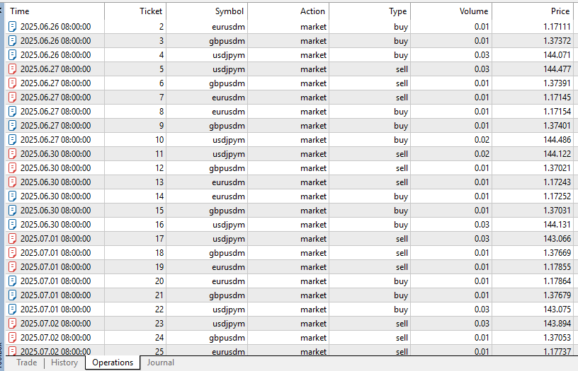
Strategy Tester deals list: the HRP Expert Advisor trading and rebalancing several instruments of the basket

Fig. 6. A Strategy Tester deals list showing the HRP Expert Advisor allocating and rebalancing across several instruments of the basket

A closing point on expectations. HRP decides how to split capital by risk, not by any forecast of return, so the Expert Advisor is an allocation engine and not a signal system. Whether a diversified, leverage-free basket makes money over a given stretch depends on the market, not on HRP. The honest way to judge it is to attach it to your own basket and timeframe in the Strategy Tester and read the result directly.

Conclusion

This article builds a Hierarchical Risk Parity allocator for MQL5 as a single class. It follows the data from raw prices to final weights without inverting the covariance matrix, verifies each stage, compares results with Markowitz on a stressed basket, and wraps the allocator into a rebalancing Expert Advisor.

CalculateReturns and BuildCovCorr turn a price panel into the covariance and correlation matrices.
HierarchicalCluster converts correlation into a proper distance and builds the single-linkage merge tree with ALGLIB.
QuasiDiagonal walks the tree to order the instruments so that similar ones sit side by side.
RecursiveBisection splits capital down the tree in inverse proportion to cluster risk.
The Expert Advisor aligns prices across instruments, sizes positions in account-currency notional, and rebalances a long-only basket.

The honest framing matters as much as the code. HRP is not a lower-variance method than Markowitz, and it makes no forecast of return. What it does produce, reliably and by construction, is a long-only, fully invested, leverage-free, interpretable allocation that never collapses into the fragile 331% gross long-short book the optimizer built on the same data. If your goal is squeezing out the last basis point of in-sample variance, mean-variance optimization is the tool. If your goal is a robust, implementable allocation you can actually hold, and a risk profile that stays stable when the covariance estimate does not, HRP is the more sensible choice. The allocator, the Expert Advisor, and the verification scripts are all attached, ready to run on your own baskets.

#	Filename	Type	Description
1	CHRPAllocator.mqh	Header	The HRP allocator, full five-stage pipeline
2	HRP_EA.mq5	Expert	Rebalancing Expert Advisor with cross-instrument time alignment
3	HRP_Export_CovCorr.mq5	Script	Runs the pipeline and exports every stage for the correctness cross-check
4	hrp_crosscheck.py	Python	Independent numpy and scipy verification of every stage
5	MQL5.zip	Archive	Archive with all the files above, ready to unpack into the terminal data directory so each file lands in its correct location

Attached files |

Download ZIP

MQL5.zip (11.22 KB)

Warning: All rights to these materials are reserved by MetaQuotes Ltd. Copying or reprinting of these materials in whole or in part is prohibited.

This article was written by a user of the site and reflects their personal views. MetaQuotes Ltd is not responsible for the accuracy of the information presented, nor for any consequences resulting from the use of the solutions, strategies or recommendations described.