Uncertainty as a Model (Part 3): Mathematical Statistics — How to Extract Knowledge from Data

Table of Contents

1. Foreword
2. Introduction
3. Fundamental Limit Theorems
1. The i.i.d. model
2. The Law of Large Numbers (LLN)
3. The Central Limit Theorem (CLT)
4. Basic Concepts and Approaches in Mathematical Statistics
1. Population
2. Sample
3. Empirical cumulative distribution function
4. Exploratory Data Analysis (EDA)
5. Confirmatory Data Analysis (CDA)
6. Parametric Methods
7. Nonparametric Methods
8. Estimation of Numerical Characteristics
9. Testing Statistical Hypotheses
5. Conclusion
6. Appendix
7. List of Attached Files

Foreword

In the previous part, we examined the framework of multivariate random variables, which allows us to describe complex relationships between assets. However, theoretical knowledge of distribution laws is merely an idealized model. In practice, a trader does not deal with the distributions themselves, but rather with their “imprints” in the form of historical data. The transition from the analysis of abstract vectors to working with real samples marks a shift from pure probability theory to the field of mathematical statistics. It is precisely here that limit theorems, such as the LLN and the CLT, serve as a bridge that allows us to infer global properties of market processes from a limited set of data.

As an example of the application of mathematical statistics, we should mention the models underlying the current AI boom — large language models (LLMs). The process of training them is a classic problem of point estimation of parameters (weights), the number of which reaches hundreds of billions. These values are found using maximum likelihood estimation, which makes even the most advanced neural networks a direct extension of traditional statistical approaches at an unprecedented data scale.

Introduction

We write trading scripts and regularly encounter the same practical problem: we have a history of price quotes, but it is unclear what in it represents a stable market characteristic and what represents a random fluctuation in a specific sample. Because of this, it's easy to mistake noise for a signal — “the mean is positive,” “there is a correlation,” “the distribution is close to normal” — and end up failing in real-world trading.

The purpose of this article is to provide a practical statistical framework for analyzing historical data: how to properly conceptualize a sample (both as a model and as specific numbers), which limit theorems (the LLN and the CLT) support conclusions for finite N, and which practical procedures can be quickly implemented in code to test distributions, estimate parameters, and distinguish statistically significant effects from illusions. In this context, the i.i.d. model is introduced not as a dogma, but as a testable hypothesis — a key focus of EDA and CDA. This article outlines the steps involved and provides examples of MQL5 scripts that can be immediately incorporated into our testing pipeline.

Fundamental Limit Theorems

Let's conclude our brief overview of probability theory with its two main results: the Law of Large Numbers (LLN) and the Central Limit Theorem (CLT). But before we move on to them, we need to define the working framework — the model in which these laws come to life.

The i.i.d. model: independent and identically distributed

The most important and frequently used model in data science is a sequence of independent and identically distributed random variables (called i.i.d., independent and identically distributed, in the English-language literature). In the theory of stochastic processes, this model serves as the foundation for the concept of "white noise." Formally, working with infinite collections of random variables belongs to the theory of stochastic processes, but traditionally it remains at the heart of probability theory. What does this mean mathematically?

1. Independence: the joint density of a set of n variables decomposes into the simple product of their individual densities: pjoint(x₁, x₂, ..., xₙ) = p₁(x₁)*p₂(x₂)*...*pₙ(xₙ)
2. Identical distribution: we assume that all variables “play by the same rules.” They have identical probability density functions, so instead of a set of different densities p₁(x₁), p₂(x₂), ..., pn(xₙ), we use a single one, denoted by p(): pjoint(x₁, x₂, ..., xₙ) = p(x₁)*p(x₂)*...*p(xₙ).

An important nuance: although all the random variables in the sequence are identically distributed, they represent different objects. You can think of this as a series of tosses of the same perfectly fair coin: the rules of the game (the distribution) are identical for each toss, but the outcome of each individual toss is a separate, independent event.

The Law of Large Numbers (LLN): From Randomness to Predictability

The Law of Large Numbers is precisely the rule that allows casinos to always stay in the black and insurance companies to avoid bankruptcy, despite the unpredictability of each individual customer. Or, conversely, to go bankrupt if the applicability conditions of the LLN are violated in a way that is unfavorable to them.

Suppose we have a sequence of N independent and identically distributed random variables Xi, each with expected value M. We define a new random variable — their arithmetic mean: Xmean = (X1 + X2 + ... + XN) / N. The essence of the law: the LLN states that as N tends to infinity, this average value ceases to be random. It “contracts” to a degenerate random variable that takes the value M with probability 1.

In other words, when summed, the individual noise of each separate random variable cancels out, leaving us with a clean, bare constant — the expected value. Example: From Probability to Frequency. The best-known consequence of the LLN is the proof that the frequency of an event approaches its probability:

1. Let us consider a series of N trials (for example, coin flips or trade entries).
2. Let Xi = 1 if the event occurred (profit or heads), and Xi = 0 if it did not.
3. The probability of success is p, and the probability of failure is 1 - p. Then the expected value of each Xi is: M = 1*p + 0*(1-p) = p.
4. The arithmetic mean in this case is simply the frequency n/N, where n is the number of successes in a series of N trials.

According to the LLN, with a large number of trades, our actual win rate, n/N, will inevitably approach the theoretical probability p.

An important conclusion for trading: the LLN is the foundation of a trading edge. If our expected value is positive, then over a long series of trades, randomness will “evaporate,” and our equity curve will inevitably converge to the expected profit. Randomness rules a single trade, but regularity governs a thousand. But let us not forget that this works only if the conditions of the LLN are met, and these conditions are by no means guaranteed to hold always and everywhere in the real world.

The Central Limit Theorem (CLT): The Architecture of Random Deviations

If the Law of Large Numbers gives us a qualitative answer to the question “What does the mean converge to?”, the Central Limit Theorem brings quantitative rigor to this process. In essence, the CLT is a deeper refinement of the LLN.

The LLN states that as N → ∞ , the arithmetic mean Xmean of independent and identically distributed random variables Xi converges to a constant — the expected value M. However, the LLN says nothing about exactly how the error of this approximation, Xmean - M, behaves on its way to the limit. The CLT fills this gap by describing the distribution of this error.

The CLT proves that, for sufficiently large (but finite!) N, this difference is not distributed arbitrarily. It turns out that the random variable Xmean - M has a distribution that is very close to a normal (Gaussian) distribution with the following parameters:

1. Zero mean: the error is symmetric about zero.
2. Variance D/N: where D is the variance of a single original variable Xi.

Let us once again emphasize the importance of the CLT for finite samples. The practical value of the theorem lies precisely in its applicability to large but finite samples. In the real world, we never reach an infinite N. The CLT allows us to rigorously calculate the probabilistic bounds within which our mean will fall for a specific, finite amount of data.

Main conclusions: (1) the rate at which the mean converges to the expected value is proportional to 1/sqrt(N); (2) the distribution of deviations of the mean from the expected value tends toward a normal distribution.

Transition to Mathematical Statistics: The designation “central” underscores the exceptional role of this theorem — it links any stochastic processes with the normal distribution. It is the CLT that gives mathematical statistics the basis for using the normal approximation to analyze real samples. Now, armed with an understanding of how theoretical randomness turns into observable patterns, we can move from probability theory to the practice of data analysis — mathematical statistics.

Basic Concepts and Approaches in Mathematical Statistics

Basic concepts include the population and the sample, as well as the division of statistics into two stages: preliminary data exploration (EDA) and drawing conclusions from the data (CDA). In turn, CDA is divided by modeling approach into parametric and nonparametric models, and by the tasks being addressed into estimation of characteristics and hypothesis testing.

Population: beyond the “bag of balls”

In elementary problems, the population can easily be visualized as a “bag of multicolored balls.” We know that there is a finite number of objects in the bag, and the population is simply a complete list of them. In this model, the sample consists of the few balls we managed to pull out.

However, for most real-world problems (and trading in particular), this analogy is hopelessly outdated. We cannot think of “all possible prices for tomorrow” as a fixed set of balls in a bag. This is where a deeper concept comes into play: the ensemble of states.

The simplest way to view the population is not as a physical set of objects, but as a probabilistic model that defines the rules of the game. This is the hypothetical “everything” that our experiment could, in principle, produce. Since we never see the entire population, it remains a theoretical ideal for us, whose properties we judge from a sample.

Sample: Two Different Concepts

It is important to note that the concept of a sample in mathematical statistics has a fundamental duality. This often becomes an obstacle when reading specialized literature:

• The sample as a result (numbers): these are the specific quotes we downloaded from the trading terminal this morning. This is a specific realization of random variables.
• A sample as a model (random variables themselves): Before the experiment is conducted, we view the sample as a set of random variables.

The sample is interesting not only in and of itself. It is typically used to calculate certain numerical indicators, which are commonly referred to as sample statistics. Depending on the context, they, too, can be regarded either as random variables or as ordinary numbers. Most of the time, it is quite clear what is being discussed, but here is a simple rule that can help with intuition: when we calculate the sample mean before the experiment, we are dealing with random variables. When we calculate it afterward, we are working with specific numbers.

Thus, a sample is a set of numerical values x₁, x₂, ..., xₙ for the random variables X1, X2, ..., Xn, obtained as a result of a random experiment. It is also very often assumed that these random variables are independent and identically distributed. However, it is not entirely correct to narrow the definition right away: this creates the mistaken impression that random variables are always independent and identically distributed. In fact, we often have to use methods of mathematical statistics to determine whether a given sample possesses these properties. And sometimes we even have to model how these assumptions are violated.

Empirical cumulative distribution function

Nevertheless, the concept of independent and identically distributed (i.i.d.) random variables remains central to the presentation of the fundamentals of statistics. The fundamental concept underlying such samples is the empirical cumulative distribution function (ECDF). Its definition: Pe(x) = k(x)/n, where k(x) is the number of sample elements less than or equal to x, and n is the total number of sample elements (sample size). The main property of the empirical cumulative distribution function is that, as the sample size increases, it approaches the true distribution function of the original random variables.

Essentially, the ECDF is an ordinary discrete cumulative distribution function with steps at the sample points. And nothing prevents us from calculating any characteristics that can be computed for distribution functions. Sometimes the original discrete version of the ECDF is not entirely suitable for further analysis, in which case a smooth approximation is constructed for it. Furthermore, for continuous distributions that have a density function, an empirical approximation of that function — known as a histogram — is constructed. Often, instead of a discontinuous histogram, its smoothed version is used, for example via kernel density estimation (KDE).

Descriptive Statistics and Exploratory Data Analysis (EDA)

In modern mathematical statistics, it is customary to divide the process into two fundamental stages: EDA (Exploratory Data Analysis) and CDA (Confirmatory Data Analysis), i.e. hypothesis-driven analysis.

Descriptive statistics are usually defined formally as the calculation of key numerical characteristics of a sample. These include the statistics we are already familiar with: the sample mean, variance, median, and quartiles. This also includes visualization — creating histograms, box-and-whisker plots (boxplots), and other graphical forms.

However, behind these dry calculations lies a crucial informal component — exploratory data analysis (Exploratory Data Analysis, EDA). The essence of EDA is to “hear the voice of the data.” This is not simply filling out a table of characteristics. This is a preliminary “probing” of the data, whose purpose is to understand its internal structure and select the appropriate mathematical framework for further study.

An example from trading. If we examine price increments, sound EDA will quickly shatter the illusion of an “ideal world.” Instead of independent and identically distributed (i.i.d.) random variables, we will discover:

• the volatility clustering effect: periods of calm are followed by spikes (dependence);
• “heavy tails”: anomalous jumps occur more frequently than a normal distribution would predict.

Why is this important? While descriptive statistics provide us with a "profile" of the sample (height, weight, age), EDA helps us understand its "character." Without this step, it is easy to make a fatal mistake: for example, applying methods that require data independence in situations where the market exhibits strong inertia or memory.

Thus, EDA is the foundation. Before building complex predictive models or testing hypotheses, we must ensure that our tools are applicable to this specific population.

The appendix to the article includes a table with several examples of functions from the standard MQL5 library for calculations used in exploratory analysis. It also provides examples of calculations and charts that are useful for a preliminary review of the data.

Confirmatory Data Analysis (CDA): From Hypotheses to Facts

While exploratory data analysis (EDA) helps us form hypotheses and identify potential patterns in the data, the subsequent phase — confirmatory data analysis (CDA) — is designed to confirm or refute those hypotheses.

This is a vast and complex field of methods designed to confirm or refute hypotheses formulated during the preliminary stage. To avoid getting lost in the wide variety of CDA tools, let’s start by making a fundamental distinction between all statistical methods, dividing them into two broad categories: parametric and nonparametric.

Parametric Statistics: Families and Their Members

Before moving on, we need to clarify the term “parametric” itself. In this field, we do not work with arbitrary distributions, but rather with strictly limited sets of them — parametric families of distributions.

What is a family? Imagine a general "template" or "blueprint" for a distribution. For example, the normal distribution is a two-parameter family. The "blueprint" itself is the same, but its specific form (the width of the "bell" and its position on the axis) depends on two numbers: the mean m and the variance s^2.

• A family is a general mathematical formula (template).
• A specific member of a family is a distribution in which specific numbers are substituted for the letters (for example, a normal distribution with a mean of 0 and a variance of 1).

A terminological pitfall: in the literature, people often take liberties by referring to the entire family as a “distribution” in the singular. For example, people say "exponential distribution," meaning the entire vast set of possible variants. But if the reference is to an "exponential distribution with a mean of two," then that points to a specific "player" from that team.

The problem of different parameterizations. Another source of headaches for an analyst is the various ways of describing the same family. While everything is always standard with the family of normal distributions, confusion often arises with other families, such as the gamma or exponential distribution. For example, the family of exponential distributions can be defined in two ways:

1. By the mean value (scale parameter m).
2. By the rate (parameter λ), with λ=1/m.

Why is this important? Different statistical packages in Python, R, or MQL5 may use different parameterizations for the same family of distributions. If we are used to thinking in terms of the "mean," but the library expects the "rate," then our probability calculation will turn out to be catastrophically incorrect. It is always a good idea to read the documentation that comes with the package.

Nonparametric Statistics: Freedom from Templates

Unlike the parametric approach, nonparametric statistics deliberately avoids being tied to specific "families" (whether normal or exponential). Here, we do not try to guess what blueprint the data were generated from; instead, we work with them "as is."

At the same time, broad classes can be used instead of rigid parametric families: giving up a specific formula does not imply a complete lack of structure. Instead of relying on membership in a specific family, we can rely on qualitative properties. For example, these could include:

• Symmetry: We assume that the left and right sides of the "bell" are mirror images of each other (though the bell itself can be any shape).
• Positivity: We know that the quantity cannot be less than zero (this applies to asset prices or volatility).
• Unimodality: We are confident that the probability density has only one pronounced peak (one mode).
• Tails: we analyze only the rate at which probability decays at the edges (the asymptotic behavior), without concerning ourselves with what happens in the center.

One of the most elegant tools of the nonparametric approach is rank-based methods. Instead of working with the sample observations themselves (which may contain wild outliers or have unusual scales), we replace them with ranks.

How does it work? We take a sample and sort it in ascending order. Each number in the sample is assigned its ordinal position — its rank. For example, a return value (say, 500%) simply becomes “the largest number in the list.” This instantly makes the analysis robust: a single extreme outlier (market manipulation or a technical error) will not “blow up” our statistics, since its rank will change only slightly.

Intuitive explanation: rank-based methods are like judging in sports, where what matters is not by how many milliseconds an athlete beat their opponent, but who came in first, second, and third. This allows us to draw reliable conclusions even when the “stopwatch” (our data) is not working perfectly.

An example of a rank-based method is the Mann–Whitney U test, which is included in the ALGLIB library (included in the MQL5 standard library).

Estimation of Numerical Characteristics: Point and Interval Estimation

Now let's shift our perspective and classify methods not by their internal structure, but by the types of problems they solve. Broadly speaking, all statistical activities can be divided into two categories: estimating the numerical parameters of models and testing assumptions (hypotheses). The difference between them lies primarily in the nature of the conclusions:

1. Estimation problems give us a specific numerical answer. For example, what is the Hurst exponent on this section of the price chart?
2. Hypothesis testing yields a qualitative, binary verdict. Here, we are not looking for a number; we are answering a question. For example, whether our fractal analysis of this section of the price chart indicates that the price is not behaving like a random walk.

Despite their different end results, both paths are based on the same probabilistic logic. Let's start with the first and most commonly used approach — Estimation of Numerical Characteristics. This is the simplest and most common scenario in data analysis: when, based on an available sample, we need to calculate a single number that will serve as the best approximation of the characteristic we are looking for:

1. The sample mean becomes an estimate of the expected value.
2. The frequency of an event is an estimate of its probability.

The main rule: never put an equals sign between a quantity and its estimate. For example, probability is a real property of the object under study (albeit within the framework of a limited model), while frequency is merely what we were able to observe in a specific experiment. As with the concept of a sample, the concept of an estimate has a dual meaning determined by context. It is both a number and a random variable. To avoid confusion in calculations, you need to clearly distinguish between these two aspects:

• An estimate as a number: this is a specific result of calculations based on data that have already been collected. We loaded 100 bars of historical data, ran the calculation, and got: "The average increment is 0.003." Here, an estimate is a number — a fixed result.
• An estimator as a random variable: before the data are obtained, the estimator is a function of the sample (a set of random variables X1, X2, ..., Xn). In this sense, it is itself a full-fledged random variable with its own distribution, expected value, and variance. In the literature, it is often called a sample statistic, or simply a statistic.

Why is this distinction critical? When we discuss the “good” properties of an estimator (consistency and so on), we refer to it exclusively as a random variable. For intuition: think of it as echolocation in fog. Let's imagine that we are on a ship trying to determine the distance to an invisible rocky shore in thick fog using sonar.

• The true value of the parameter: the actual distance to the shore. The shore exists; it is a certain distance away from us, but we cannot see it.
• The estimator is a random variable: our device itself, its calibration, and the algorithm it uses.
• An estimate is a number: a single, specific reading taken by an instrument. Due to interference and waves, it may show 50 meters, even though the shore is actually 70 meters away. And even if one of the measurements turns out to be accurate, we still cannot know that for sure.

The following requirements, above all, apply to an estimator as a random variable:

• Consistency (convergence at infinity). This is the minimum basic requirement for an estimator. If we keep increasing the sample size indefinitely (N → ∞), our estimator must, in the limit, coincide with the true value. Mathematically, this is expressed as convergence of the estimator to a degenerate random variable in which all probability is concentrated at the true value of the parameter being estimated.
• Unbiasedness (correctness on finite data). In reality, we do not have an infinite amount of data. It is important to us that, even with a small sample, our estimator be free of systematic error. Mathematically, this means that the expected value of the estimator is equal to the parameter being estimated.

An example of consistency: the Law of Large Numbers (LLN) guarantees that the sample mean is a consistent estimator of the expected value.

An example of unbiasedness: people are often surprised that the denominator in the formula for the sample variance is N-1, rather than the more intuitive N. The answer lies precisely in the requirement of unbiasedness. The point is that if we do not know the true expected value, we are forced to substitute its estimate (the sample mean) in its place. Dividing by N would yield a slightly underestimated result (a biased estimator). This can be seen by calculating the expected value of the estimator. The one-unit correction in the denominator is a mathematical adjustment that makes the variance estimator unbiased.

A fundamental method for finding point estimates is maximum likelihood estimation. It is based on the likelihood function — the same probability density function (or probability in the discrete case), but considered not as a function of the data, but as a function of the unknown model parameters for a fixed sample. In this case, the problem boils down to finding the parameter values that make the observed data the most likely.

The appendix to this article contains MQL5 scripts for calculating point estimates of the expected value, variance, median, interquartile range, and several types of correlation coefficients.

Since any point estimate based on a finite sample is a random variable, it inevitably has its own variance. In other words: there will always be some variation in the results of our experiments, and therefore some error as well. In physics, when measuring the length of a part, it is customary to specify the precision: “1.2 m ± 5 mm.” We do not just give a number; we define an interval within which we believe the true value lies. In mathematical statistics, we proceed in a similar manner, but with some fundamental differences:

• No 100% guarantee. Unlike in physics, in statistics we can never guarantee with 100% certainty that the true value falls within a given interval. There is always a slim chance that we ended up with an anomalous sample that misled us. Therefore, along with the interval, we always specify the confidence level — the probability that our method has “covered” the true parameter. That is precisely why this interval is called a confidence interval. It is very common to choose standard confidence levels of 95% or 99%.
• A trade-off between precision and confidence. The interval and the confidence level are inextricably linked. If we want to raise our confidence level to 100%, our confidence interval will begin to widen until it becomes infinite (for example: “Tomorrow’s price will be between zero and infinity” — a statement that is true but useless).

The job of an analyst is always about finding a balance:

• We want the interval to be as narrow as possible (high precision).
• We want the confidence level to be as high as possible (high reliability).

However, these desires pull in opposite directions. To narrow the interval while maintaining high reliability, we have only one way: increase the sample size.

The appendix to this article contains MQL5 scripts for calculating interval estimates of the mean, median, and correlation coefficients.

Testing Statistical Hypotheses

The basic logic behind hypothesis testing was discussed earlier in the article on elementary (discrete) probability theory. In the world of random variables, it remains fully valid. The main difference here is the enormous variety of methods, which is simply impossible to cover in a single article. To avoid getting lost in this sea of tests, let's divide the hypotheses into two broad (albeit overlapping) classes:

1. Hypotheses about model applicability. Here, we test global assumptions about the structure of the data. Example: “Does the sample come from a normal distribution?”, “Were these two samples drawn from independent random variables?”. These are tests of the “adequacy” of the chosen mathematical framework. For example, if the normality hypothesis is rejected, then all subsequent calculations based on the parameters of this family lose their meaning.
2. Hypotheses regarding numerical characteristics. Unlike a simple estimate (which gives us a number), here we are testing specific statements. For example, instead of asking, “What is the expected value?” we ask: “Is it true that the expected value of the return is strictly greater than zero?” or “Is the correlation between assets equal to zero?” Why this is needed: a simple point estimate (for example, a mean of 0.0001) does not, on its own, answer the question of whether this result is a genuine signal or simply random noise in the data. Hypothesis testing allows us to filter out results that are not statistically significant.

These two classes of methods are not isolated from one another. We often reject an entire model precisely because its key parameter has turned out to be zero (for example, we reject a model of a linear relationship if the correlation coefficient is statistically indistinguishable from zero).

When studying methods for testing hypotheses, it is important not to get confused by the terminology. In the Russian mathematical tradition, the algorithm we use to reach a conclusion (“whether to reject the hypothesis or not”) is commonly referred to as a statistical criterion. In English-language contexts — and, more importantly, in program code — the word “test” is almost always used. This distinction is critical for practical work:

• In a Russian-language textbook, we would read about the classic Kolmogorov–Smirnov goodness-of-fit test.
• In English-language documentation, this is referred to as the Kolmogorov–Smirnov test (or KS test for short).
• In code — for example, in R — the corresponding function would be called `ks.test()`.

From the user's perspective, working with any statistical test usually boils down to a standard sequence of steps. The entire path from data to a decision consists roughly of the following steps:

1. Formulation of hypotheses. We always deal with a pair: H0 (null) — the hypothesis of no effect (the market is random, there is no relationship) and H1 (alternative) — the statement we want to prove. At this stage, it is critically important to understand exactly what the selected test is assessing, so as not to end up with the “right answer to the wrong question.”
2. Choosing the significance level α. As with confidence intervals, there is no 100% guarantee. The significance level is our own “tolerance threshold” for a Type I error (the risk of falsely rejecting a true H0). Even if we use the “default” settings in software (0.05 or 0.01), we need to remember: this choice always remains ours.
3. Calculating the test statistic and finding the critical region. Each test has its own statistic (sample statistic). Based on the selected significance level α and the distribution of this statistic, a critical region is determined — a zone of “extreme” values that are too unlikely in a world where H0 is true.
4. If the numerical value of the statistic calculated from our sample falls within the critical region, we are justified in rejecting the null hypothesis H0 at the specified significance level.
5. If the value does not fall within the critical region, we do not reject H0. Important: This does not prove that H0 is true. It simply means that we do not have sufficient data to refute it. The test does not allow us to reject H1; it simply leaves us at the status quo.
6. Using the p-value. Modern software often saves us the trouble of looking up critical regions in tables by returning a computed p-value. The rule here is simple: if p-value < α, then the null hypothesis H0 is rejected.

To avoid getting lost among the hundreds of existing hypothesis-testing methods, let us identify the two main categories on which most modern research is based. For each of them, we will give several examples of specific tests:

1. Goodness-of-Fit Tests

Their purpose is to check how well our sample fits the chosen theoretical model. We ask: “Do these data look like what the formula predicts?”

• The Kolmogorov–Smirnov test (KS test) is a classic tool for determining whether a sample follows a specific distribution, for example, a normal distribution with given parameters.
• Pearson’s chi-square test is used to assess the discrepancy between observed frequencies and expected probabilities.
• The Shapiro–Wilk test is one of the most powerful statistical tests for testing the hypothesis of normality of the sample distribution. Its key difference from the Kolmogorov–Smirnov test is that it does not test whether the data are close to a specific distribution function with given parameters, but rather whether they belong to the family of normal distributions.

2. Tests for Dependence

These tests look for hidden relationships between different variables or within a single time series.

• A correlation significance test checks whether the relationship between assets is genuine or merely a random coincidence.
• The Durbin–Watson test detects autocorrelation (for example, a relationship between the current price and its past values), which is critical for identifying trends.
• Tests based on mutual information are a modern approach for identifying any nonlinear relationships — even the most unusual ones — that conventional correlation fails to detect.

The appendix to this article contains MQL5 scripts for testing hypotheses regarding expected value, the median, and correlation coefficients.

Conclusion

We now have a concrete, basic framework for analyzing historical price data and a set of practical skills that can be immediately applied to strategy development. Specifically, we have learned how to / are now able to:

1. Correctly define the population and interpret the sample in two ways (as a model and as observed data).
2. Construct the empirical cumulative distribution function (ECDF) and perform basic EDA to identify heavy tails, outliers, and autocorrelation.
3. Compare standard and robust point estimates and construct confidence intervals based on the LLN and the CLT (error ≈ 1/sqrt(N)).
4. Formally test hypotheses (normality, zero mean/median, absence of dependence) and decide whether to proceed with parametric methods or switch to nonparametric/robust techniques if the assumptions are not met.

The appendices contain MQL5 scripts and example charts that implement this pipeline. Limitations: details of maximum likelihood estimation and the Bayesian approach are omitted here — this is the next logical step. In our upcoming publications, we will continue with: first, stochastic processes (for modeling price dynamics), then more advanced estimation methods and Bayesian techniques. For now, let's incorporate the suggested checks into our workflow — this will significantly reduce the risk of mistaking noise for a signal and improve the reliability of our decisions in the live market.

Appendices: Practical Implementation in Code

All of the examples provided in the appendix are intended solely for educational purposes and have been deliberately simplified to clearly illustrate mathematical concepts. The material presented here does not contain any direct trading ideas or investment recommendations.

Appendix 1

A table listing some statistical functions from the standard MQL5 library for calculating sample statistics.

Function Name	Function
Empirical cumulative distribution function (ECDF)	MathCumulativeDistributionEmpirical()
Sample density of a continuous distribution	MathProbabilityDensityEmpirical()
Sample quantiles	MathQuantile()
Sample mean	MathMean()
Sample variance	MathVariance()
Sample correlation (Pearson)	MathCorrelationPearson()
Calculation of sample ranks (for rank-based methods)	MathRank()

Appendix 2

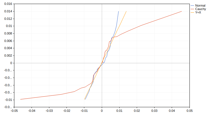
The qqplot.mq5 script, which constructs Q-Q plots for visually comparing the distribution of a sample of price changes with the Cauchy and Gaussian distributions. This graph clearly shows that the Cauchy distribution is much less suitable for modeling price behavior.

Appendix 3

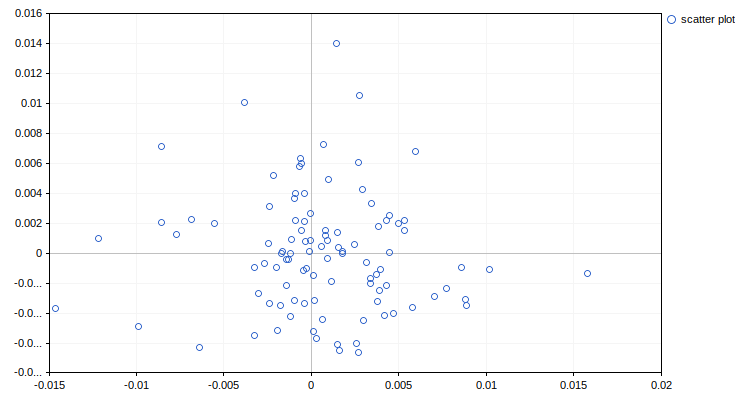
The scatter_plot.mq5 script for visualizing relationships in price movements. It constructs a scatter plot whose axes represent successive price changes at the current step and at the next step. This plot allows you to visually assess the strength of the statistical relationship between past and future market movements. In our case, no significant relationship is apparent; otherwise, the points would be noticeably clustered around a particular line.

Appendix 4

The point_est.mq5 script performs point estimation of parameters of a normal distribution for price changes in two ways: the standard method and the robust method (using the median and the interquartile range). In our case, there is a noticeable difference between the two estimates (the robust standard deviation is nearly one and a half times smaller). This indicates the need to test the sample for normality (for example, using the Shapiro–Wilk test). Calculation results:

Estimation of the parameters of a normal distribution using two methods
1) Using the sample mean and standard deviation:
For the expected value: 0.00013, for the standard deviation: 0.00433
2) Using the sample median and interquartile range:
For the expected value: -0.00042, for the standard deviation: 0.00301

Appendix 5

The conf_est.mq5 script calculates interval estimates of the expected value and median for a sample of price changes. Calculation results:

Sample mean: 0.00033
Sample median: 0.00011
Expected value interval: from -0.00026 to 0.00092, with a confidence level of 0.950
Median interval: from -0.00041 to 0.00080, with a confidence level of 0.950

Note: At the time this article was written, the MathQuantileT() library function had a bug. Therefore, line 32 is commented out, and the replacement function MathQuantileT_TMP() is called below.

Appendix 6

The H_mean.mq5 script tests the hypotheses that the expected value and median of the distribution of price changes are equal to zero. Calculation results:

Sample mean: 0.00033
Sample median: 0.00011
The null hypothesis that the expected value is equal to zero is NOT rejected at a significance level of 0.05
The null hypothesis that the median is equal to zero is NOT rejected at a significance level of 0.05

Appendix 7

The H_corr.mq5 script calculates three different types of correlation coefficients (Pearson, Spearman, and Kendall) between successive price changes and tests the hypotheses that all three coefficients are equal to zero. Calculation results:

Sample Pearson correlation coefficient: -0.068
Sample Spearman correlation coefficient: -0.093
Sample Kendall correlation coefficient: -0.061
The null hypothesis that the Pearson correlation coefficient is equal to zero is NOT rejected at a significance level of 0.05
The null hypothesis that the Spearman correlation coefficient is equal to zero is NOT rejected at a significance level of 0.05
The null hypothesis that the Kendall correlation coefficient is equal to zero is NOT rejected at a significance level of 0.05

Attached Files

#	name	Description
1	qqplot.mq5	A script that generates Q-Q plots for a visual comparison of the sample distribution of price changes with the Cauchy and Gaussian distributions.
2	scatter_plot.mq5	A script for visualizing the dependence between successive price changes.
3	point_est.mq5	A script for computing point estimates for the parameters of the normal distribution in two ways
4	conf_est.mq5	A script for calculating interval estimates for the expected value and median of a sample of price changes.
5	H_mean.mq5	A script for testing the hypotheses that the expected value and median of the distribution of price changes are equal to zero
6	H_corr.mq5	A script for calculating three different types of correlation coefficients (Pearson, Spearman, and Kendall) and for testing the hypotheses that all three coefficients are equal to zero.