

Which Economic Releases Actually Move Your Symbol, and by How Much?
 635
 0

Introduction
The usual way to handle an economic release inside an Expert Advisor is to treat it as a category. It has a name, a currency, a scheduled time, and an importance flag, and the standard thing to do with it is to stand aside: block trading for thirty minutes either side of anything marked high impact. The only tuning available is the importance threshold and the width of the window, and neither of those has anything to do with the release itself.
But a release is not a category. It is a number arriving against an expectation. Two payrolls prints can share the same importance flag, the same currency and the same clock time, and one of them will move EURUSD fifty pips inside a minute while the other barely registers. The calendar does carry a directional label for each release, in the impact_type field of every calendar value, so the platform is not silent on the question. What a label cannot express is how far, and how far is the whole difference between those two prints.
The quantity that separates them is the surprise: the actual figure minus the forecast, scaled so that it means the same thing across indicators measured in completely different units. In this article we build that quantity in MQL5, and then we measure what it actually does to price.
Three properties of the data have to be handled before any of that is trustworthy, and every one of them is easy to miss. We will find all three by measurement rather than assumption, because each silently produces a plausible-looking answer that is wrong.
We will cover:
- What the Calendar Actually Carries
- From a Category to a Number
- Anchoring a Release to the Bar That Moved
- The Engine
- Measuring the Response
- Reading It on a Chart
- What the Numbers Say, and What They Do Not
- Conclusion
What the Calendar Actually Carries
The raw material is MqlCalendarValue. Each row is one release of one event and carries an actual value, a forecast, a previous value, a period, and a revision index. Any of the three values may be absent, and the methods HasActualValue, HasForecastValue and HasPreviousValue tell you which.
Before building anything on top of this, it is worth knowing how much of it there is. We measured the depth directly by walking every high-importance event on the eight major currencies.

Fig. 1. The terminal's own calendar window, showing the three values every row may carry
The result sets the scope of what follows. Forecast history begins in May 2017, platform-wide. Actual values go back roughly twenty years further, so any analysis built on actual minus forecast is limited by the forecast series. That leaves around 110 usable releases for each major monthly US indicator and 486 for Initial Jobless Claims, which is weekly.
One finding here changes the shape of the whole article. The entire central bank family carries no forecast values at all. The Fed interest rate decision has zero usable rows, and so do the ECB, the BoJ and the RBNZ; the Bank of England has five, all from 2017 and 2018. Speeches and press conferences are of type CALENDAR_TYPE_EVENT and carry no numbers at all. A surprise cannot be computed where no consensus was ever recorded, so rate decisions are out of scope here and we say so plainly rather than quietly producing nothing for them.
Eurozone coverage is thin for the same reason. Almost every high-importance EUR entry is ECB commentary with no values attached, leaving CPI y/y and little else. On EURUSD it is the dollar leg that carries the analysis.
From a Category to a Number
The surprise is the deviation from consensus:
s_i = actual_i - forecast_i
Raw, this is useless across indicators. Payrolls surprises are measured in thousands of jobs and run to the hundreds; CPI surprises are measured in tenths of a percentage point and run to about 0.3. There is no sense in which a payrolls surprise of 120 is larger or smaller than a CPI surprise of 0.2. To compare them we divide each by the spread of that indicator's own past surprises:
z_i = (s_i - location) / spread
Now both are in units of "how unusual is this, for this indicator", and a reader can say that one release was a two sigma surprise and another was a quarter of a sigma, and mean something by it.

Fig. 2. Two different events, the same flag, two incomparable raw surprises, two comparable standardised values
The obvious choice for location and spread is the mean and the standard deviation. On this data that choice fails badly, and finding out why produced the first real result of the project.
The forecast series carries values that cannot be real. Among the payrolls rows is a consensus of 78,356 thousand jobs, and another of minus 76,324. Consensus figures reach the terminal from an upstream data provider, and a handful of them arrive mis-scaled. These are not large surprises, they are impossible ones. The median absolute payrolls surprise over the sample is 120 and the ninetieth percentile is 601, while the largest is 77,695, which is roughly 650 times the median and 130 times the ninetieth percentile.
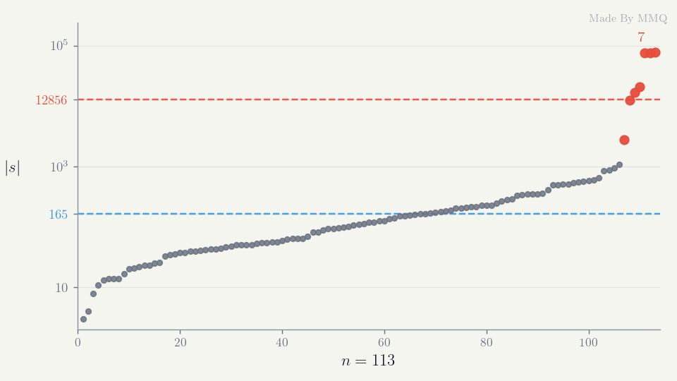
Fig. 3. Every absolute payrolls surprise, sorted. The robust scale is 165; the naive standard deviation over the same rows is 12,856
A standard deviation computed over that sample comes out at 12,856. Divide a real surprise of 120 by 12,856 and you get 0.009, so every genuine release in the sample is standardised into indistinguishable noise by a handful of bad rows. This is exactly the failure mode that makes an analysis look finished and produce nothing.
The fix is a robust pair: the median for location, and the median absolute deviation scaled by 1.4826 for spread, which makes it consistent with the standard deviation under normality. The class offers all three estimators so the difference can be seen rather than asserted.
//--- how the surprise dispersion is estimated.
enum ENUM_SURPRISE_STD
  {
   SURPRISE_STD_FULL,                  // whole sample; descriptive only
   SURPRISE_STD_EXPANDING,             // prior releases only; no look-ahead
   SURPRISE_STD_ROBUST                 // prior releases, median and MAD
  };
Note what separates the last two from the first. A full-sample scale uses releases that had not happened yet at the time each earlier release printed, which is look-ahead bias. The expanding and robust modes compute location and spread from strictly prior releases only, so a z printed on the day is a number that could genuinely have been known on the day.
Neither mode can standardise its first releases, because there is no prior history to scale against. SURPRISE_MIN_PRIOR holds the first twenty back and leaves their z empty. That warm-up is why the release counts in the previous section and the n column of the results later do not match: an event with 110 usable rows contributes 90 points to a regression, not 110. Every number reported in this article was produced in SURPRISE_STD_ROBUST, which is what all three attached programs default to.
//+------------------------------------------------------------------+
//| Location and spread of the surprises before index upto: median   |
//| and MAD, so a corrupt forecast cannot crush every real z.        |
//+------------------------------------------------------------------+
void CCalendarSurprise::Scale(const int upto,double &location,double &spread) const
  {
   location = 0.0;
   spread   = 0.0;
   if(upto <= 1)
      return;

   double s[];
   ArrayResize(s, upto);
   for(int k = 0; k < upto; k++)
      s[k] = m_rel[k].surprise;

   if(m_mode == SURPRISE_STD_ROBUST)
     {
      location = Median(s, upto);
      double dev[];
      ArrayResize(dev, upto);
      for(int k = 0; k < upto; k++)
         dev[k] = MathAbs(s[k] - location);
      spread = 1.4826 * Median(dev, upto);
      return;
     }

   double sum = 0.0;
   for(int k = 0; k < upto; k++)
      sum += s[k];
   location = sum / upto;

   double ss = 0.0;
   for(int k = 0; k < upto; k++)
      ss += (s[k] - location) * (s[k] - location);
   spread = MathSqrt(ss / (upto - 1));
  }
A robust scale stops those rows from inflating sigma, but it does not remove them. Left in the sample they now arrive as several hundred sigma each, and a single point at four hundred sigma dominates any regression it appears in. They have to be gated out explicitly, and counted while we are at it, because how many there are is itself worth reporting. The gate is SURPRISE_MAX_Z, set to ten: past ten sigma on a robust scale a row is a data error rather than a surprise. This excerpt closes Standardise:
   m_event.n_corrupt = 0;
   for(int i = 0; i < m_count; i++)
     {
      if(m_rel[i].z == EMPTY_VALUE || MathAbs(m_rel[i].z) <= SURPRISE_MAX_Z)
         continue;
      m_rel[i].z      = EMPTY_VALUE;
      m_rel[i].reject = SURPRISE_BAD_FORECAST;
      m_event.n_corrupt++;
     }
  }
Across the eleven US indicators we track, the gate removes 53 rows. They are concentrated in the employment and retail families; the CPI and ISM families come through clean.
That split is also why the gate is not discarding real shocks. A genuine shock is economy wide, so a gate catching shocks would catch them in inflation too, and the CPI, Core CPI, Core PCE and both ISM series lose nothing at all across the whole sample, 2020 included. Ten robust sigma is not a large surprise, it is an impossible one.
Anchoring a Release to the Bar That Moved
Knowing the surprise is half the job. The other half is knowing which minute of price to compare it against, and this turns out to be where most of the difficulty lives.
The calendar's stamped release time does not reliably sit on the bar that moved. We found this by scanning the M1 bars either side of each stamp and asking where the largest absolute minute return actually was. On a release big enough to dominate its own window, that offset should be zero. It frequently was not.
There are two separate causes, and they need separate fixes.
The first is a synchronisation race. Reading the calendar repeatedly from a freshly started terminal shows the answer changing under you:
poll 0 (0 ms,    connected=0):  CPI m/m -> 2017.05.12 12:30
poll 1 (3360 ms, connected=1):  CPI m/m -> 2017.05.12 15:30
Same event id, same query, two different answers three seconds apart. Before the terminal connects, the calendar returns stamps in GMT; after it connects, it returns them in server time. On a GMT+3 server that is a 180-minute shift, and it flips silently mid-run. A script that reads the calendar during startup gets timestamps three hours from where its bars are, with no error anywhere.
The gate for this has to be usable from an indicator, which rules out sleeping. Indicators run on the interface thread and Sleep is refused there, so the check holds no state between calls and can simply be asked again on the next tick.
//+------------------------------------------------------------------+
//| One non-blocking check that the calendar can be trusted.         |
//| Holding no state lets OnCalculate use it, where Sleep() is out.  |
//+------------------------------------------------------------------+
bool CCalendarSurprise::CalendarProbe(void)
  {
   if(!TerminalInfoInteger(TERMINAL_CONNECTED))
      return(false);

   const ulong probe = 840030016;      // US Nonfarm Payrolls; always populated
   MqlCalendarValue a[], b[];
   int na = CalendarValueHistoryByEvent(probe, a, D'2017.01.01', TimeCurrent());
   int nb = CalendarValueHistoryByEvent(probe, b, D'2017.01.01', TimeCurrent());

   if(na <= 0 || na != nb)
      return(false);
   return(a[0].time > 0 && a[0].time == b[0].time);
  }
The second cause is daylight saving. Once connected, the calendar answers in server time, which is the right frame in which to compare a stamp against server bars. Server time, though, carries its own daylight saving schedule, and a historical stamp expressed with today's offset lands an hour from its own bar whenever the release sits on the far side of a changeover. Which releases are affected therefore depends on when you happen to be reading, and reconciling it is the caller's job rather than something the calendar can decide on your behalf.

Fig. 4. The stamp, the bar that actually moved, and the offset between them
The important design point is whose property this is. The size of the shift belongs to the broker's server clock, not to any individual indicator. Our first attempt calibrated an offset per event, and it was visibly wrong: one event offers only about nine releases per month, few of which dominate their window, so ambiguous months fell back to a default and the two ISM events ended up disagreeing about which months shift. They release on the same clock, so they cannot both be right.
Pooling fixes it. CCalendarClock calibrates once from every release of every tracked event. It needs only actual values, not forecasts, because alignment depends on whether a release moved the market and not on whether anyone predicted it. That makes the voting pool larger than the pool usable for standardisation.
Each release votes for the offset of the largest absolute minute return near its stamp, but only if that move stands out from the window around it: the peak has to clear SURPRISE_DOMINANCE, eight times the median minute of the window. A quiet release has nothing to say about where the clock sits, and letting it vote would be letting noise vote. The window is the study's InpScan, four hours either side, which is wide enough to contain even the three hour shift the first cause can produce.
//+------------------------------------------------------------------+
//| Offset of the largest absolute minute return around one stamp.   |
//| counted stays false when no move stands out: a quiet print.      |
//+------------------------------------------------------------------+
int CCalendarClock::Vote(const string symbol,const datetime stamp,
                         const int scan_minutes,bool &counted) const
  {
   counted = false;
   double point = SymbolInfoDouble(symbol, SYMBOL_POINT);
   if(point <= 0.0)
      return(0);

   datetime a = stamp - scan_minutes * 60;
   datetime b = stamp + scan_minutes * 60;

   double o[], c[];
   datetime t[];
   int n = CopyOpen(symbol, PERIOD_M1, a, b, o);
   if(n <= 0 || CopyClose(symbol, PERIOD_M1, a, b, c) != n ||
      CopyTime(symbol, PERIOD_M1, a, b, t) != n)
      return(0);

   double mv[];
   ArrayResize(mv, n);
   double peak = -1.0;
   int    arg  = 0;
   for(int k = 0; k < n; k++)
     {
      mv[k] = MathAbs(c[k] - o[k]) / point;
      if(mv[k] > peak)
        {
         peak = mv[k];
         arg  = (int)((t[k] - stamp) / 60);
        }
     }

   ArraySort(mv);
   double median = mv[n / 2];
   if(median <= 0.0 || peak / median < SURPRISE_DOMINANCE)
      return(0);

   counted = true;
   return(arg);
  }
Votes are bucketed by the month the release falls in. A month adopts its own answer only when enough releases agreed on it, at least CLOCK_MIN_VOTES of them, and that answer is the size a daylight saving shift can be: within SURPRISE_OFFSET_BAND, ninety minutes, of m_global, the modal offset over the whole pool. Without that second condition a handful of quiet releases can carry a month somewhere impossible, which is exactly what happened in an early run where ADP came back with a 105 minute offset for September on three weak votes.
   for(int m = 0; m < 12; m++)
     {
      int best = -1;
      for(int k = 0; k < nv[m]; k++)
         if(best < 0 || tally[m][k] > tally[m][best])
            best = k;

      bool trust = (best >= 0 && tally[m][best] >= CLOCK_MIN_VOTES &&
                    MathAbs(offs[m][best] - m_global) <= SURPRISE_OFFSET_BAND);
      m_month[m] = (trust ? offs[m][best] : m_global);
      m_votes[m] = (best >= 0 ? tally[m][best] : 0);
     }
What comes back is a textbook daylight saving schedule, with 24 to 60 votes behind each month.
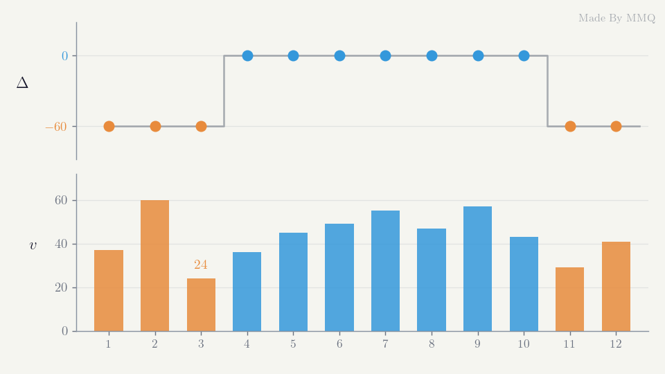
Fig. 5. The offset recovered for each month, and the number of releases that voted for it
Nothing in the code knows what daylight saving is. There is no timezone table, no hard-coded changeover date, and no assumption about which hemisphere the server is in. The schedule falls out of the price, and it is worth pausing on that: the same method will recover a different and equally correct table on a broker whose server keeps a different clock.
The figure also reports its own weakest point rather than hiding it. March carries only 24 votes because it straddles the changeover date and genuinely contains releases on both sides of it. A calendar month is the wrong granularity exactly there, and the vote count says so.
The Engine
With the scale and the clock settled, the engine itself is small. CCalendarSurprise holds one event: its descriptor, its releases, and the standardised surprise for each.
//+------------------------------------------------------------------+
//| One release: the raw numbers, the surprise, and its anchor.      |
//+------------------------------------------------------------------+
struct SurpriseRelease
  {
   datetime          stamp;            // exactly as the calendar reported it
   datetime          anchor;           // stamp moved onto the bar that moved
   datetime          period;           // the period the figure describes
   double            actual;
   double            forecast;
   double            previous;
   double            surprise;         // actual - forecast, native units
   double            z;                // standardised; comparable across events
   int               reject;           // ENUM_SURPRISE_REJECT
  };
Loading has one subtlety that matters more than its size suggests. The calendar stores revisions: the same period can appear several times as the statistical agency restates it. The news, though, is the first print, because that is the number the market actually traded. A later revision must never overwrite it, so among the rows sharing a period we keep the one carrying the lowest revision index, breaking a tie on the earlier stamp. Selecting on the revision rather than on the order the rows arrive in matters more than it looks: the terminal does return them oldest first, but nothing in the API promises that, and a first-print rule that quietly depends on it would be wrong without ever failing visibly.
      int slot = -1;
      for(int k = 0; k < m_count && slot < 0; k++)
         if(m_rel[k].period == v[i].period)
            slot = k;
      if(slot >= 0 && (v[i].revision > held[slot] ||
                       (v[i].revision == held[slot] &&
                        v[i].time >= m_rel[slot].stamp)))
         continue;                     // the row already held is earlier

      SurpriseRelease r;
      ZeroMemory(r);
      r.stamp    = v[i].time;
      r.anchor   = v[i].time;
      r.period   = v[i].period;
      r.actual   = v[i].GetActualValue();
      r.forecast = v[i].GetForecastValue();
      r.previous = (v[i].HasPreviousValue() ? v[i].GetPreviousValue() : 0.0);
      r.surprise = r.actual - r.forecast;
      r.z        = EMPTY_VALUE;
      r.reject   = SURPRISE_OK;

      if(slot >= 0)
        {
         m_rel[slot] = r;
         held[slot]  = v[i].revision;
        }
      else
        {
         held[m_count]    = v[i].revision;
         m_rel[m_count++] = r;
        }
The measurement itself is a regression of the signed price move on the standardised surprise, through the origin. That constraint is a modelling choice rather than a fact about releases. A print carries revisions and component figures that a single headline surprise does not summarise, so a zero headline surprise is not literally guaranteed to be zero news. What the constraint does say is that we are unwilling to let the fit absorb whatever drift happened to sit in the sample through a free intercept, because that drift has nothing to do with the surprise. The slope is then directly interpretable as pips per sigma of surprise.
Because this assumption matters, we tested it: we refitted all 176 cells with a free intercept and compared the results. Not one intercept survives a false discovery rate correction, and the 10 that clear an uncorrected threshold sit close to the 8.8 expected by chance alone. The median fitted intercept is 2.1 pips, against first-minute moves of around twenty pips on the largest releases. The two fits rank the cells almost identically, with a correlation of 0.99 between their t statistics, and across the cells significant under the constraint the slope shifts by a median of 2.8 percent and never changes sign: Core CPI on EURUSD moves from -7.55 pips per sigma to -7.40. The constraint is costing us nothing, which is the only defence of it worth making.
//+------------------------------------------------------------------+
//| Regress the signed move on the standardised surprise, through    |
//| the origin: the intercept is held at zero, not estimated.        |
//+------------------------------------------------------------------+
bool CCalendarSurprise::Response(const string symbol,const int horizon_min,
                                 SurpriseResponse &out)
  {
   ZeroMemory(out);
   out.symbol      = symbol;
   out.horizon_min = horizon_min;

   double point = SymbolInfoDouble(symbol, SYMBOL_POINT);
   int    digits = (int)SymbolInfoInteger(symbol, SYMBOL_DIGITS);
   if(point <= 0.0)
     {
      m_error = "no point size for " + symbol;
      return(false);
     }
   double pip = ((digits == 3 || digits == 5) ? point * 10.0 : point);

   double xs[], ys[];
   ArrayResize(xs, m_count);
   ArrayResize(ys, m_count);
   int n = 0;
   double abs_sum = 0.0;

   for(int i = 0; i < m_count; i++)
     {
      if(m_rel[i].z == EMPTY_VALUE)
         continue;

      datetime a = m_rel[i].anchor;
      //--- the stop time is inclusive: end a second early, h bars not h+1.
      datetime b = a + horizon_min * 60 - 1;

      double o[], c[];
      datetime t[];
      int k = CopyOpen(symbol, PERIOD_M1, a, b, o);
      if(k <= 0 || CopyClose(symbol, PERIOD_M1, a, b, c) != k ||
         CopyTime(symbol, PERIOD_M1, a, b, t) != k)
         continue;
      if(MathAbs((long)(t[0] - a)) > SURPRISE_BAR_SLACK)
         continue;                     // no bar at the anchor; market shut

      double move = (c[k - 1] - o[0]) / pip;
      xs[n] = m_rel[i].z;
      ys[n] = move;
      abs_sum += MathAbs(move);
      n++;
     }

   if(n < 10)
     {
      m_error = StringFormat("only %d usable releases for %s", n, symbol);
      return(false);
     }

   double sxy = 0.0, sxx = 0.0, syy = 0.0;
   for(int i = 0; i < n; i++)
     {
      sxy += xs[i] * ys[i];
      sxx += xs[i] * xs[i];
      syy += ys[i] * ys[i];
     }
   if(sxx <= 0.0)
     {
      m_error = "zero surprise variance";
      return(false);
     }

   double slope = sxy / sxx;

   double rss = 0.0;
   for(int i = 0; i < n; i++)
     {
      double e = ys[i] - slope * xs[i];
      rss += e * e;
     }
   double se = (n > 1 ? MathSqrt((rss / (n - 1)) / sxx) : 0.0);

   out.n              = n;
   out.slope          = slope;
   out.stderr         = se;
   out.t_stat         = (se > 0.0 ? slope / se : 0.0);
   out.r2             = (syy > 0.0 ? 1.0 - rss / syy : 0.0);
   out.mean_abs_move  = abs_sum / n;
   out.band_spans_zero = (MathAbs(out.t_stat) < 1.96);
   return(true);
  }
One line in the loop decides what a horizon means. A copy by start and stop time returns every bar whose open falls inside the range, both ends included, so a stop of exactly anchor plus h minutes would bring back h + 1 bars and a one-minute horizon would quietly measure two. Ending the range a second early returns exactly h bars, the anchor bar included, so the move runs from the open of the anchor bar to the close h minutes later.
The band_spans_zero flag is the one a reader should care about most, and it is worth being precise about what it says. When the confidence band on the slope includes zero, this regression has found no linear directional response for this indicator on this symbol at this horizon. That is narrower than it sounds. A response confined to the tails, or one that differs between beats and misses, can sit inside a flat overall slope, and a single slope through the origin is not built to see it. What a flat row does warn against is searching for a threshold in-sample until one works: every cut tried is another test, and a cut chosen that way needs its own correction for the search before it counts as evidence.
Every judgement the engine makes is governed by a named constant rather than a number buried in a condition, and they are worth having in one place.
| Constant | Value | What it decides |
|---|---|---|
| SURPRISE_MIN_PRIOR | 20 | Releases held back before a z can be standardised at all |
| SURPRISE_MAX_Z | 10 | Beyond this many sigma, a row is treated as a data error and rejected |
| SURPRISE_BAR_SLACK | 120 | Seconds a bar may sit from its anchor before the release is skipped as market-shut |
| SURPRISE_DOMINANCE | 8.0 | Peak over median a release must clear before it may vote on the clock |
| SURPRISE_OFFSET_BAND | 90 | Minutes a month's offset may differ from the pooled mode and still be trusted |
| CLOCK_MIN_VOTES | 5 | Votes a month needs before it sets its own offset instead of inheriting the pooled one |
Measuring the Response
SurpriseLab runs the whole thing: it settles the calendar, calibrates the clock once, then loads each event, anchors it, and fits a response for every symbol and horizon requested. A script may block, so it waits with WaitForCalendar, which wraps the probe from the previous section in the Sleep loop an indicator cannot use.
   if(!CCalendarSurprise::WaitForCalendar(60000))
     {
      Emit(h, "FATAL,calendar did not settle within 60s");
      FileClose(h);
      return;
     }

   string syms[], hors[];
   int nsym = StringSplit(InpSymbols,  ',', syms);
   int nhor = StringSplit(InpHorizons, ',', hors);
   for(int s = 0; s < nsym; s++)
      SymbolSelect(syms[s], true);

   string modes[3] = {"full", "expanding", "robust"};
   Emit(h, StringFormat("standardiser,%s,scan_minutes,%d", modes[(int)InpMode], InpScan));
//--- one clock for the whole run: DST belongs to the server.
   CCalendarClock clock;
   if(!clock.Calibrate(syms[0], EventIds, InpScan, D'2017.01.01', TimeCurrent()))
      Emit(h, "CLOCK WARNING," + clock.LastError());
The machinery is in place; what follows is what it returned. Run over eleven US indicators, four symbols (EURUSD, GBPUSD, USDJPY and XAUUSD) and four horizons (one, five, fifteen and sixty minutes) on M1 data from May 2017, 46 of the 176 cells (event × symbol × horizon) clear a two-sided test at the five percent level.
That number has to be read against how many cells a five-percent threshold hands out for free. Testing 176 cells against a null of no response would be expected to produce about nine, and 46 is far above that. The excess cannot be turned into a probability, though, because the cells are not independent: the sixteen cells of one event share the same releases, the four symbols answer to the same dollar news, and each shorter horizon is part of every longer one. Under that kind of dependence one real effect can light up a whole block of cells at once, so the count says there is structure here without saying how many separate effects carry it. Individual cells are the stricter question.
A Benjamini and Hochberg false discovery rate correction at five percent keeps ten cells, and all ten are Core CPI. The far harsher Bonferroni bound keeps five, all Core CPI again, and Bonferroni needs no assumption about how the tests depend on one another: whatever the dependence, the chance that it admits even one false cell is at most five percent. That is what the claim of a real response rests on.
This matters, because it limits how much weight we can place on any single row. That a response exists is settled, the inflation family is individually solid, and the middle of the table is a set of cells that clear an uncorrected threshold without surviving a correction for how many thresholds were crossed. We report them as measured, not as established.
The clearest result is Core CPI, and what makes it convincing is not the size of the slope but its behaviour across symbols.
| Symbol | Slope, pips per sigma | Std. error | t | R^2 |
|---|---|---|---|---|
| EURUSD | -7.55 | 1.77 | -4.28 | 0.170 |
| GBPUSD | -8.30 | 2.08 | -3.98 | 0.151 |
| USDJPY | +10.92 | 3.20 | +3.41 | 0.141 |
| XAUUSD | -211.08 | 78.30 | -2.70 | 0.093 |
A hot inflation print strengthens the dollar. On EURUSD, GBPUSD and XAUUSD the dollar is the quote currency, so the pair falls and the slope is negative. On USDJPY the dollar is the base, so the pair rises and the sign flips. Nothing in the engine knows which currency sits on which side of a symbol; it regresses a price move on a number. That the sign inverts on exactly the one symbol where it should is a genuine check, and a cheap one to fail. It does not validate the data quality, the anchoring or the statistical model, each of which is argued for separately above; what it validates is that the sign we measure is the sign the market actually delivered, rather than an artifact of how the pairs are quoted.
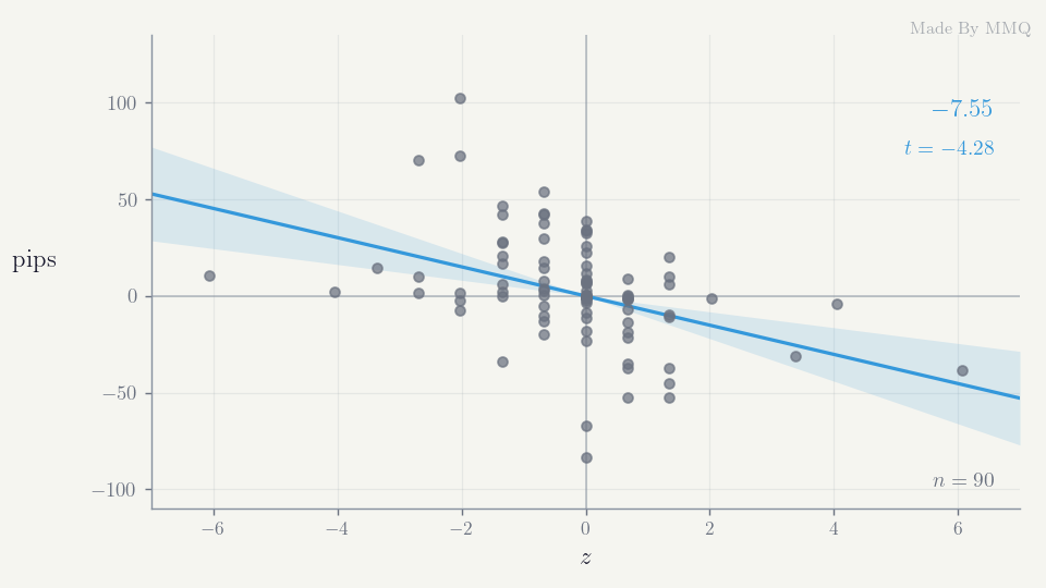
Fig. 6. The Core CPI response on EURUSD one minute after the print, with the through-origin fit and its confidence band
The points in Fig. 6 sit on a visible lattice. That is not a plotting artifact: Core CPI month on month is published to one decimal place, so the raw surprise is always a multiple of 0.1 and the standardised value inherits that granularity. It is a genuine feature of the data and worth seeing rather than smoothing away.
Extending the fit across horizons shows something a single number would hide.
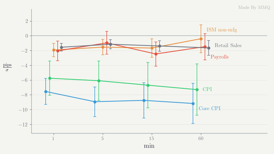
Fig. 7. Slope against horizon on EURUSD, with one standard error either side
The inflation response does not decay over the hour. Whatever the market does in the first minute is still there at the end of the sixtieth, which is a different statement from the response simply being large. It is also a statement about endpoints only: each horizon measures the move from the anchor to that horizon, so this says nothing about the path in between, and a cumulative slope that holds up is entirely compatible with reversals inside the window. The near zero group behaves quite differently, and holding longer does nothing to rescue it.
Finally, the anchoring work from earlier can be priced. We ran the identical study twice, once against raw calendar stamps and once against anchored ones, changing nothing else.
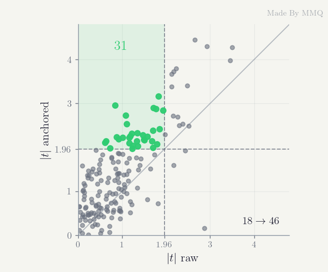
Fig. 8. Every response cell measured twice. The shaded block holds the cells that only become detectable once the release is anchored
Eighteen of the 176 cells clear the threshold on raw stamps. Forty six clear it once anchored, and mean absolute t rises from 0.94 to 1.40. No data was added and no parameter was tuned between those two runs. The entire gain comes from measuring the response in the right minute, which is a useful reminder that a negative result can be an artifact of the plumbing rather than a fact about the market.
The correction from the previous section sharpens that comparison rather than blunting it. Eighteen cells out of 176 is close enough to what a five-percent threshold produces by chance that the raw stamp run yields no discoveries at all once the false discovery rate is controlled. The anchored run yields ten. The honest way to price the anchoring work is therefore not eighteen cells against forty six, but nothing against ten: before the release is placed on the bar that moved, there is no evidence here that survives being counted properly.
Reading It on a Chart
Two programs put the measurement on a chart. SurpriseMeter is the instrument proper: a separate window plotting the standardised surprise of whichever release landed on each bar, zero everywhere else, with the magnitude and the originating event id exposed as calculation buffers so an Expert Advisor can read them through iCustom.
Buffer 2 carries the magnitude and buffer 3 the event id that produced it, so the whole hook on the Expert Advisor side is a handle and two copies:
   int h = iCustom(_Symbol, PERIOD_M1, "CalSurprise\\SurpriseMeter");
   double mag[], id[];
   if(CopyBuffer(h, 2, 0, 1, mag) == 1 &&
      CopyBuffer(h, 3, 0, 1, id)  == 1 && mag[0] >= 2.0)
      PrintFormat("event %I64u printed %.2f sigma", (ulong)id[0], mag[0]);
The second buffer is what makes the first one usable. A magnitude on its own says only that something unusual landed; paired with the id, the Expert Advisor knows which indicator surprised and can treat a two sigma CPI print differently from a two sigma jobless claims print. The zero on every other bar is deliberate rather than an empty value, because a bar with no release genuinely carries no surprise. Both copies return short until the indicator has cleared its own calendar gate, so an Expert Advisor should treat a failed copy as not ready yet rather than as an absent release.
Two constraints shaped it, both of them consequences of running on the interface thread.
The first is that placement has to be cheap. A naive implementation rescans every release for every bar, which on a long M1 chart is well over a hundred million comparisons and freezes the terminal outright. Since both the releases and the bars are sorted, a binary search per release is enough.
//+------------------------------------------------------------------+
//| Index of the last bar opening at or before t, or -1. Binary      |
//| search; rescanning every release per bar would stall the UI.     |
//+------------------------------------------------------------------+
int BarIndexOf(const datetime t,const datetime &time[],const int total)
  {
   if(total <= 0 || t < time[0])
      return(-1);
   int lo = 0, hi = total - 1;
   while(lo < hi)
     {
      int mid = (lo + hi + 1) / 2;
      if(time[mid] <= t)
         lo = mid;
      else
         hi = mid - 1;
     }
   return(lo);
  }
The second is the calendar gate. We measured the full load and calibration of all eleven events at 63 milliseconds, so there is nothing to gain by spreading it over ticks; what cannot be done is blocking while waiting for the calendar to settle.
   if(!Ready)
     {
      if(!CCalendarSurprise::CalendarProbe())
         return(0);

      //--- the clock is shared, so calibrate it once for all events.
      CCalendarClock clock;
      clock.Calibrate(_Symbol, Ids, InpScan, D'2017.01.01', TimeCurrent());
      for(int i = 0; i < ArraySize(Ids); i++)
         LoadOne(Ids[i], clock);
      SortReleases();
      Ready = true;
     }

Fig. 9. SurpriseMeter on EURUSD H2, each release standing on its own bar with the colour carrying the sign of the surprise
SurprisePanel answers the forward looking question instead: for each release still to come, what has this indicator historically done to this symbol. Each row carries the countdown, the fitted slope, its t statistic, the mean absolute move, and the last realised surprise. Rows whose confidence band spans zero are dimmed, so a glance separates the releases whose past response was measurable from the ones that only look important. What the panel forecasts is nothing: every number in it is history, and it ranks the calendar by how legible each indicator has been rather than by what any of them is about to do. The surprise itself does not exist until the actual prints.
The panel is driven from OnTimer rather than OnCalculate, and that is not a stylistic choice. A quiet market delivers no ticks, and a panel that only woke on ticks would sit blank all weekend, which is precisely when someone is most likely to be reviewing the week ahead.
//+------------------------------------------------------------------+
//| Settle the calendar, rebuild on a slow cadence, and redraw       |
//| every timer tick so the countdown stays live.                    |
//+------------------------------------------------------------------+
void OnTimer(void)
  {
   if(!Ready)
     {
      if(!CCalendarSurprise::CalendarProbe())
        {
         Draw();
         return;
        }
      Build();
      LastBuild = TimeCurrent();
      Ready     = true;
     }
   else if(TimeCurrent() - LastBuild >= InpReload)
     {
      Build();
      LastBuild = TimeCurrent();
     }

   Draw();
  }

Fig. 10. SurprisePanel, with flat rows dimmed against the ones carrying a measurable response
What the Numbers Say, and What They Do Not
Here is the one-minute response on EURUSD for every indicator we tracked.
| Indicator | n | Slope, pips per sigma | t | Mean abs. move |
|---|---|---|---|---|
| Core CPI m/m | 90 | -7.55 | -4.28 | 19.6 |
| Retail Sales m/m | 89 | -1.55 | -2.96 | 7.9 |
| ADP Nonfarm Employment Change | 83 | -0.79 | -2.72 | 5.6 |
| CPI m/m | 90 | -5.75 | -2.49 | 19.6 |
| Core Retail Sales m/m | 86 | -1.10 | -2.28 | 8.0 |
| Initial Jobless Claims | 446 | +0.60 | +2.19 | 5.5 |
| ISM Non-Manufacturing PMI | 90 | -1.93 | -2.14 | 7.6 |
| Nonfarm Payrolls | 85 | -2.04 | -1.52 | 22.3 |
| ISM Manufacturing PMI | 90 | -1.14 | -1.25 | 6.5 |
| Core PCE Price Index m/m | 89 | -0.40 | -0.87 | 4.5 |
| Unemployment Rate | 88 | +0.87 | +0.62 | 21.6 |
Only the ends of this ranking are firm. Core CPI clears the correction from the previous section; the group between it and the flat rows, from Retail Sales m/m down to ISM Non-Manufacturing PMI, does not, and is worth re-measuring on your own feed rather than trusted as six established effects.
The row worth the most attention is not at the top. Nonfarm Payrolls is flat on every symbol and every horizon we tested: across all sixteen of its cells, the largest absolute t statistic reaches only 1.52. It is flat while moving EURUSD 22.3 pips on average in the release minute, 23.7 on GBPUSD and 37.6 on USDJPY. The market unquestionably reacts to payrolls; what it does not do is react in proportion to the standardised payrolls surprise.
That result survived every fix in this article. It is not the impossible rows, which were gated out. It is not the alignment, because the anchored run is the one reported. We record it as a finding rather than explaining it away, and note two plausible readings for anyone who wants to take it further: the payrolls release publishes several headline numbers simultaneously, including revisions to prior months that are not in the consensus at all, so the single surprise we compute may simply be the wrong summary of what arrived; and the establishment and household surveys can point in opposite directions on the same morning.
The contrast with inflation is the practical content of the table. Core CPI moves EURUSD by a comparable average amount to payrolls, 19.6 pips against 22.3, and yet one of them is predictable in sign and magnitude from the surprise while the other is not. An importance flag cannot express that difference, because the two releases carry the same flag. Importance answers the question of how closely a release is watched, which is a real and useful question, but it is not the same question as how far this release moves this symbol. The measured response profile is the complement to the flag, not a correction of it.
Reproducing any of this is a matter of running SurpriseLab on your own terminal, against whatever M1 history your broker serves back to May 2017; everything above came from a GMT+3 server on the four symbols named earlier. Retargeting it is a matter of the EventIds array, which holds the eleven US ids and nothing else. CalendarEventByCurrency will list the ids for whichever currency you would rather track, and the only requirement the engine places on an event is that its rows carry forecasts.
Several limits are worth stating plainly.
- This is a coincident measure, not a forecast. It tells you how large a move a given surprise has historically been associated with. It says nothing about the direction of the next bar, and an R^2 near 0.17 on the best indicator means most of the variation in the release minute is still unexplained.
- A calendar month is the wrong granularity at a daylight saving boundary. March contains releases on both sides of the changeover and its vote count in Fig. 5 is the lowest of the year. Sub-monthly buckets would fix the boundary and cost evidence everywhere else, which on this sample size is a bad trade.
- The sample is one broker's history and eleven US indicators. The clock is recovered from each server's own prices, so the method transfers even though the table does not; the response estimates are symbol- and feed-specific and should be re-measured rather than copied.
- The standard errors are the textbook ones. Release minute returns are heteroscedastic, heavy-tailed, and clustered on the days when several indicators print together, and the four symbols and four horizons of a single event are far from independent of one another. None of that is corrected for. It affects how precisely a t statistic should be read rather than the sign or the size of a slope, and it is why the corrected counts above matter more than any single cell.
- The clock is calibrated on the whole history at once. That is the right thing to do when describing what a server's offsets were, and it is what makes 24 to 60 votes per month possible. It does mean a release is anchored using an offset that later releases helped establish, so the calibration is not a simulation of what was knowable on the day. The standardiser is the part that is held strictly to prior releases only.
- There is no out-of-sample test here. Every number is an in-sample description of one history. Nothing has been held back to confirm that the responses persist, so these are measurements of what happened rather than evidence about what will happen.
Conclusion
We set out to replace a categorical view of economic releases with a continuous one, and to find out whether the resulting number is worth anything. The instrument is a standardised surprise, comparable across indicators measured in different units, exposed as a per-bar buffer any Expert Advisor can read.
- The surprise carries the news the release was expected to settle. Standardising by each indicator's own dispersion puts payrolls and CPI on one scale, which is what makes a threshold such as two sigma mean the same thing everywhere. That scale is a scale of magnitude: it says how unusual a print was, not what it meant, and the economic direction of a given sign still belongs to the indicator, since a hot inflation print and a hot jobless claims print pull the dollar opposite ways. Nor is a single headline figure the whole of a release, as the payrolls result below shows.
- Three properties of the data each silently ruin the measurement if unhandled. The calendar answers in GMT until the terminal connects and in server time afterwards; server time carries its own daylight saving schedule, so a historical stamp expressed with today's offset can sit an hour from its bar; and the forecast series carries a few impossible values that destroy a scale built on the mean and standard deviation. All three produce plausible-looking output, which is exactly why each has to be found by measurement.
- The server clock belongs to the server. Pooling every release of every event recovers the broker's daylight saving schedule from price alone, with no timezone table anywhere in the code. Anchoring on that schedule lifts detectable responses from 18 cells to 46 out of 176, and, once the false discovery rate is controlled, from none at all to ten, with no other change.
- Inflation carries a measurable response and payrolls does not. Core CPI is significant on all four symbols tested, with the sign correctly inverting on USDJPY, and it is the only indicator here whose cells survive a false discovery rate correction across all 176 tests. Payrolls is flat everywhere despite moving price at least as far on average, and flat against this single headline surprise, which is a statement about the feature as much as about the release.
- A flat row is a result. Where the confidence band spans zero, this model detects no linear directional response for that symbol at that horizon, in this sample. It is the absence of a detected effect, not proof that no rule on that surprise could work, and a threshold found by searching such a row needs a correction for the search before it is evidence.
The natural next step, for anyone wanting to take this further, is the shape of the response rather than its slope: whether it saturates beyond two sigma, and whether misses and beats are symmetric. Both questions are answerable with the engine as it stands, by replacing one regression.
Getting the Source Code via MQL5 Algo Forge
All source files are attached to this article below, but the full repository is also available on MQL5 Algo Forge, the community's Git-based platform for sharing and collaborating on trading projects.
| File name | Description |
|---|---|
| MQL5\Include\CalSurprise\CalSurpriseTypes.mqh | Shared vocabulary: the event, release and response structures, and the standardiser and rejection enumerations |
| MQL5\Include\CalSurprise\CalSurpriseClock.mqh | CCalendarClock, which recovers the broker's daylight saving schedule from price by pooling votes across every tracked release |
| MQL5\Include\CalSurprise\CalSurpriseCore.mqh | CCalendarSurprise: the calendar settling gate, first-print loading, robust standardisation with an impossible-forecast gate, and the response regression |
| MQL5\Scripts\CalSurprise\SurpriseLab.mq5 | The study script: calibrates the clock, then reports the server clock, the per-event summary and the response table as CSV |
| MQL5\Indicators\CalSurprise\SurpriseMeter.mq5 | Separate-window indicator plotting the standardised surprise per bar, with magnitude and event id exposed for iCustom |
| MQL5\Indicators\CalSurprise\SurprisePanel.mq5 | Chart panel listing upcoming releases with their measured response profile, dimming those whose band spans zero |
Warning: All rights to these materials are reserved by MetaQuotes Ltd. Copying or reprinting of these materials in whole or in part is prohibited.
This article was written by a user of the site and reflects their personal views. MetaQuotes Ltd is not responsible for the accuracy of the information presented, nor for any consequences resulting from the use of the solutions, strategies or recommendations described.


