

Symbolic Fourier Approximation in MQL5: Benchmarking SFA Against SAX
 617
617
 0
0

Introduction
Turning a window of prices into a short string of letters is an old and useful trick. Once a 48-bar window is a word like dbccbdab, you can index it, count it, hash it, and compare millions of windows without touching the raw prices again. Symbolic Aggregate approXimation (SAX) does exactly this, well enough that it has become the default answer whenever somebody wants to symbolize a price series.
Every symbolic representation spends a fixed budget: a word of w letters over an alphabet of a symbols carries w · log2(a) bits per word, plus, for a representation that learns its bin table, that table stored once. Which raises a question almost nobody asks: are those bits being spent well? Most implementations pick w and a by feel, run with them, and never find out.
To find out, this article builds Symbolic Fourier Approximation (SFA), which keeps a window's low-frequency Fourier coefficients instead of its time-domain averages and learns a separate quantization table for every position. We implement it in pure MQL5, verify it against its defining identities to machine precision, and then put it head to head with SAX under a measurement harness that reports four numbers for any (w, a) you care to try.
Readers of the BOSS article have met this Fourier front end before, but BOSS classifies histograms of words and never needed a distance bound. This article adds what turns the front end into a pruned similarity search: a sound lower bound with its factor of two, an ablation that measures what the learned bins are worth, and a harness that runs SAX and SFA over identical windows.
The result, reported as it came out: SFA's advantage is large when the budget buys a deep alphabet over few positions, and it shrinks to nothing as the budget is spread over many shallow ones. SAX came out ahead in no configuration we tested. By the end you will know where the advantage lives, how much of it the learned bins supply, and you will have the harness to check it on your own symbol.
We will cover:
- Where SAX Spends Its Bits
- The Fourier Front End
- MCB: Learning the Bins
- The Lower Bound and Its Factor of Two
- From Words to Precedents
- Verifying It Works
- SAX vs SFA on Identical Windows
- The Indicator
- Conclusion
Where SAX Spends Its Bits
SAX builds a word in three steps. It z-normalizes the window so that shape survives and price level does not. It runs Piecewise Aggregate Approximation (PAA), replacing each of w equal cells with its mean. Then it maps every cell mean to a letter using breakpoints that cut the standard normal into a equal-probability bands. The last two steps each hide an assumption.
The first assumption is that averaging is a good way to compress. PAA is a boxcar filter: a reasonable summary, but not the best one. If you may keep only l numbers about a window and want the least-squares closest reconstruction, the optimal linear choice is the principal-component (Karhunen-Loève) basis of the data. When energy sits at low frequencies, as it does in price windows, the leading Fourier coefficients come close to that optimum, which is why we prefer them to block means here; on a signal with high-frequency energy, low-pass truncation would keep the wrong coefficients. The DCT and wavelets are legitimate candidates too, but this article compares the two front ends the symbolic methods in question actually use. PAA also has a subtler cost: a boxcar filter has sidelobes, so high-frequency content partly folds back into the cell mean.
The second assumption is that one bin table fits every position. SAX applies the same Gaussian breakpoints to every cell, which is defensible for PAA cells, since after z-normalization they all have roughly the same spread. Averaging does shrink a cell mean's spread below the unit variance the table assumes, so SAX draws its outer letters less often, a detail that matters less than it looks when we measure noise, but the mismatch is the same at every position. Fourier coefficients are not interchangeable: on trending price data the first coefficient carries several times the spread of the fourth. Apply one table to both and the quiet position collapses into a single letter, spending real bits on nothing.
SFA changes both steps. It replaces PAA with a truncated Discrete Fourier Transform, and the fixed Gaussian table with Multiple Coefficient Binning (MCB), one table per position, learned from data. The rest of this article builds those two changes, proves the result still supports a sound lower bound, and measures whether the changes were worth making.
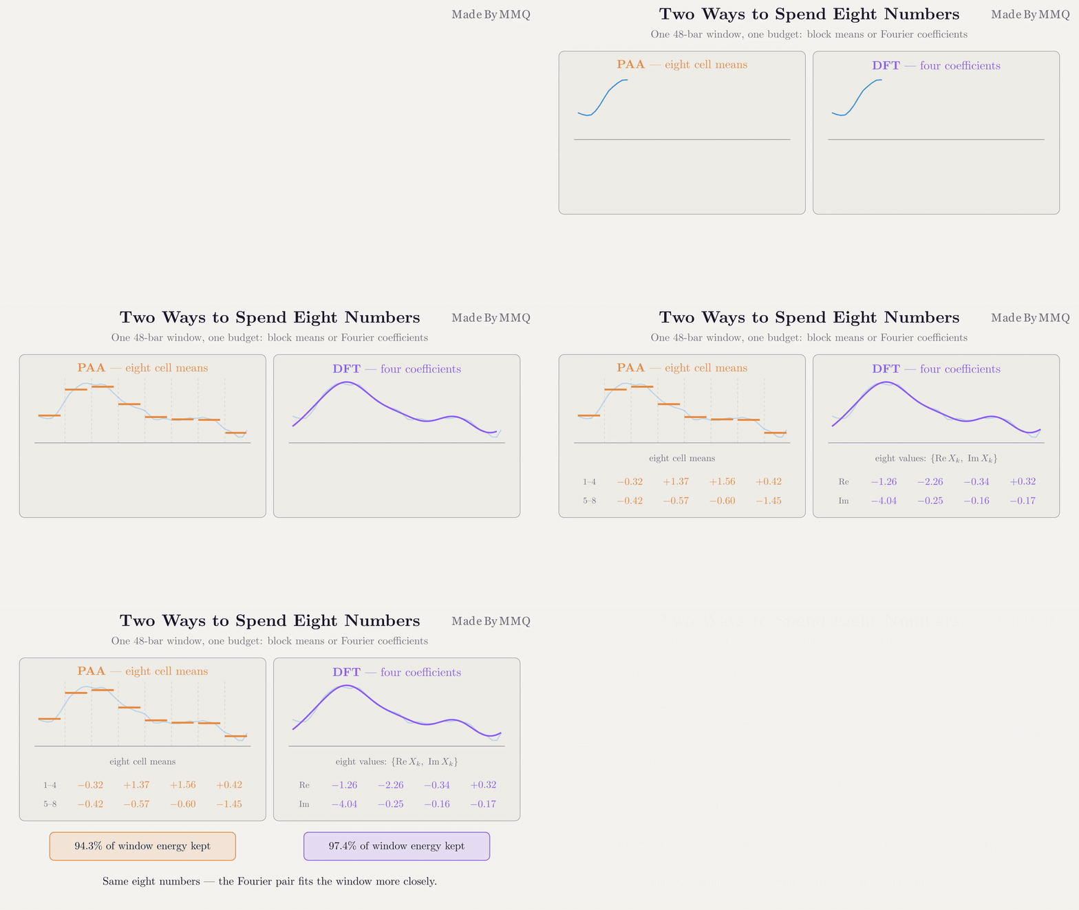
Fig. 1. The same 48-bar window compressed two ways: eight PAA cell means, and eight numbers from the first four Fourier coefficients
The Fourier Front End
The transform is bound to one window length at configuration time, because the Fourier basis depends on it. Given a window of n bars we z-normalize, then keep Discrete Fourier Transform coefficients 1 through l/2. Coefficient zero is skipped: it is proportional to the window mean, which z-normalization has already forced to zero, so retaining it would waste two of our l values on a number we know in advance. Each retained coefficient contributes its real and imaginary parts, so l/2 coefficients give exactly l values, which is why the word length must be even.
The scaling matters. Folding 1/sqrt(n) into the basis makes the transform orthonormal, so Parseval's theorem is an equality and, over the full spectrum, distances in coefficient space equal distances in the z-normalized series. The stored vector keeps only one coefficient of each conjugate pair, so its distances need one bookkeeping factor, derived in the lower-bound section.
//+------------------------------------------------------------------+
//| Precompute the DFT twiddle factors for coefficients 1..m_ncoef.  |
//|  The 1/sqrt(n) scale is folded in here, so the transform is      |
//|  orthonormal and Parseval holds without a second pass.           |
//+------------------------------------------------------------------+
void CSFATransform::BuildTwiddles(void)
  {
   ArrayResize(m_cos,m_ncoef*m_len);
   ArrayResize(m_sin,m_ncoef*m_len);

   double scale=1.0/MathSqrt((double)m_len);
   for(int c=0;c<m_ncoef;c++)
     {
      int    k=c+1;                  // coefficient index; DC is skipped
      int    base=c*m_len;
      double w=2.0*M_PI*(double)k/(double)m_len;
      for(int t=0;t<m_len;t++)
        {
         m_cos[base+t]= MathCos(w*t)*scale;
         m_sin[base+t]=-MathSin(w*t)*scale;
        }
     }
  }
With the basis cached, the transform itself is a pair of dot products per coefficient.
//+------------------------------------------------------------------+
//| Raw window -> approximation vector.                              |
//|                                                                  |
//|  Only the m_ncoef coefficients we actually keep are evaluated, so|
//|  this is O(n*l/2) rather than the O(n log n) of a full FFT. With |
//|  n=48 and l=8 that is 192 inner steps of two multiply-adds each; |
//|  a full FFT would cost more and then discard 90% of its output.  |
//+------------------------------------------------------------------+
ENUM_SFA_STATUS CSFATransform::Approximate(const double &raw[],int len,
                                           double &vec[]) const
  {
   if(!m_ready || len!=m_len)
      return SFA_BAD_PARAMS;

   double z[];
   if(!ZNormalize(raw,len,z))
      return SFA_FLAT_WINDOW;

   ArrayResize(vec,m_word);
   for(int c=0;c<m_ncoef;c++)
     {
      int    base=c*m_len;
      double re=0.0;
      double im=0.0;
      for(int t=0;t<m_len;t++)
        {
         re+=z[t]*m_cos[base+t];
         im+=z[t]*m_sin[base+t];
        }
      vec[2*c]  =re;
      vec[2*c+1]=im;
     }
   return SFA_OK;
  }
Note what is not here: an FFT. The BOSS implementation called ALGLIB's real FFT, which is the right tool when you want the whole spectrum and can afford a library dependency. Here we want four coefficients out of the forty-eight a full transform would hand back, and evaluating those four directly is cheaper and easier to read than computing all of them and discarding ninety percent.
Being cheaper than an FFT does not make it cheaper than SAX, and it is worth being straight about that. PAA reduces a 48-bar window with 48 additions; the transform spends 192 inner steps of two multiply-adds each, roughly eight times the arithmetic, and MCB adds a one-off fitting pass on top. At these sizes that is microseconds per window and it will not be what limits you; the efficiency argument this article makes is about bits, not cycles.
The output vector is laid out as {Re X1, Im X1, Re X2, Im X2, ...}, the numeric object SFA quantizes, exposed publicly so callers can inspect it rather than take the letters on faith.
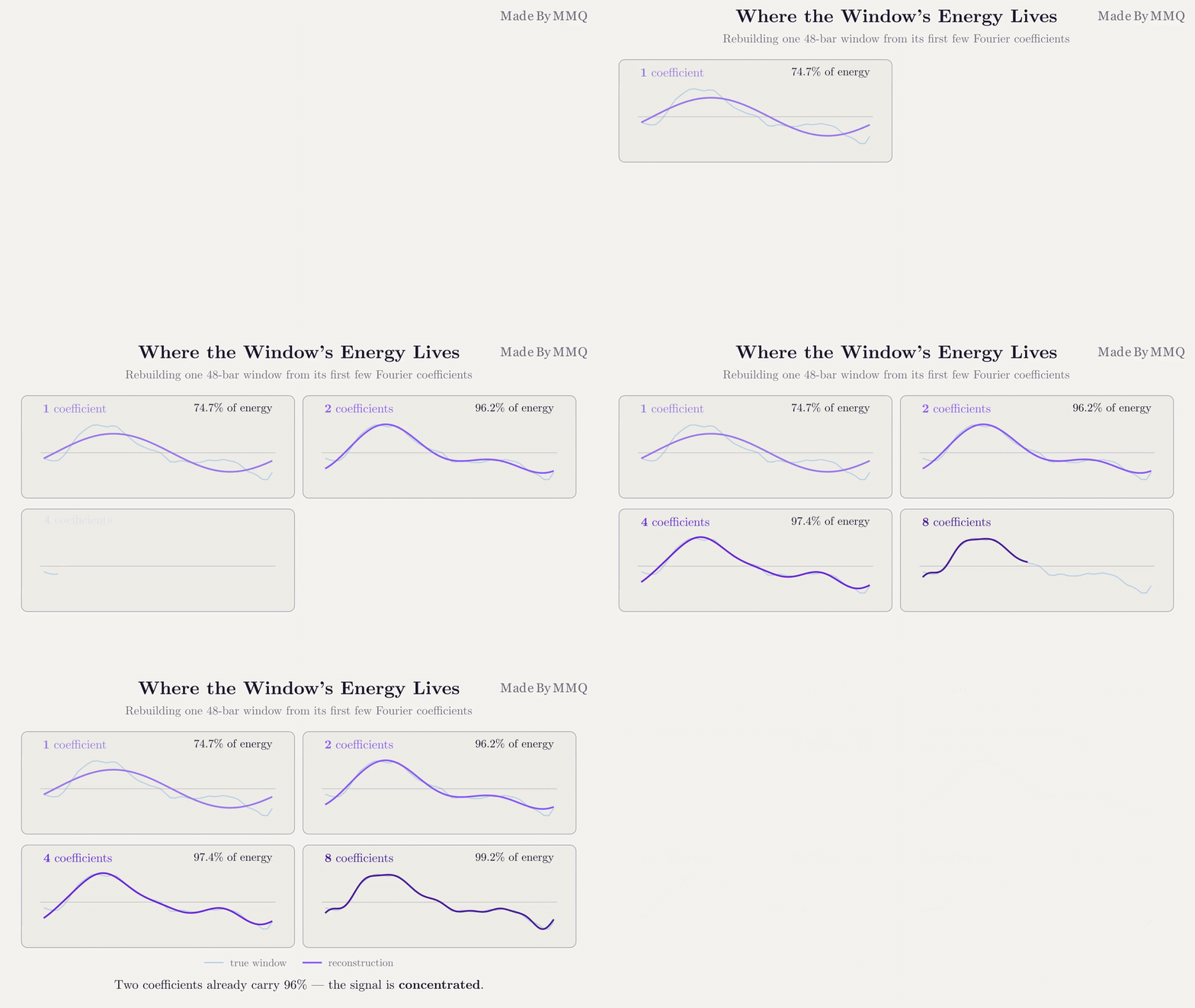
Fig. 2. Reconstructing a price window from its first one, two, four, and eight Fourier coefficients
MCB: Learning the Bins
We now have l real numbers per window, and turning each into a letter is where SFA departs from SAX most sharply. After z-normalization a window's total energy is fixed, and on price data nearly all of it sits in the lowest frequencies. The real part of coefficient 1 ranges over several units, while the imaginary part of coefficient 4 rarely leaves a narrow band around zero. Feed both to the same Gaussian breakpoints and the second lands in the middle band almost every time. It contributes a letter that is almost always the same letter, which is to say it contributes nothing while still costing its share of the bit budget.
Multiple Coefficient Binning fixes this by fitting the breakpoints per position: collect each position's values across training windows, sort them, and cut at the a-1 quantiles. On the fitting sample every letter then occurs with probability 1/a at every position, up to ties, which is the definition of using the alphabet. Out of sample the frequencies drift as the data drifts from the fit, a point the indicator section returns to.
//+------------------------------------------------------------------+
//| Turn the collected vectors into per-position bin edges.          |
//|                                                                  |
//|  EQUI_DEPTH sorts each position's values independently and cuts  |
//|  at the a-1 quantiles, so each letter is drawn with probability  |
//|  1/a. EQUI_WIDTH splits the observed range into equal intervals. |
//|  GAUSSIAN ignores the sample entirely and was already built at   |
//|  Configure() time.                                               |
//+------------------------------------------------------------------+
bool CSFATransform::FitEnd(void)
  {
   if(!m_ready)
      return false;
   if(m_binning==SFA_BINS_GAUSSIAN)
      return true;
   if(m_fitn<m_a)
      return false;                  // fewer samples than bins requested

   ArrayResize(m_beta,m_word*(m_a-1));

   double col[];
   ArrayResize(col,m_fitn);
   for(int j=0;j<m_word;j++)
     {
      for(int i=0;i<m_fitn;i++)
         col[i]=m_fit[i*m_word+j];
      ArraySort(col);

      if(m_binning==SFA_BINS_EQUI_DEPTH)
        {
         for(int i=0;i<m_a-1;i++)
            m_beta[j*(m_a-1)+i]=Percentile(col,m_fitn,
                                           (double)(i+1)/(double)m_a);
        }
      else
        {
         double lo=col[0];
         double hi=col[m_fitn-1];
         double step=(hi-lo)/(double)m_a;
         for(int i=0;i<m_a-1;i++)
            m_beta[j*(m_a-1)+i]=lo+step*(i+1);
        }
     }

   EnforceMonotone();
   m_fitted=true;
   return true;
  }
Three binning modes are supported, and the third exists purely so that the article can measure what MCB is worth. SFA_BINS_EQUI_DEPTH is MCB proper. SFA_BINS_EQUI_WIDTH splits the observed range into equal intervals, the obvious thing to try, and lets a single outlier starve the middle bins. SFA_BINS_GAUSSIAN applies SAX's fixed probit cuts to every position and serves as the ablation: same Fourier front end, wrong bin table.
A learned table can also degenerate in a way a fixed one cannot, which one small guard handles.
//+------------------------------------------------------------------+
//| Guarantee non-decreasing edges within every position.            |
//|                                                                  |
//|  A degenerate position, one whose values are heavily tied, can   |
//|  produce two identical or (through floating point) inverted      |
//|  quantiles, which would make a cell gap negative. CellDist clamps|
//|  such a gap to zero, so the bound survives either way; what this |
//|  pass buys is an edge table that still reads as a partition, at  |
//|  the cost of a wasted symbol.                                    |
//+------------------------------------------------------------------+
void CSFATransform::EnforceMonotone(void)
  {
   for(int j=0;j<m_word;j++)
     {
      int base=j*(m_a-1);
      for(int i=1;i<m_a-1;i++)
         if(m_beta[base+i]<m_beta[base+i-1])
            m_beta[base+i]=m_beta[base+i-1];
     }
  }
Because the bins are learned, we can measure whether they are used. BinOccupancy histograms the fitted sample across a position's bins, and the validation script reports the worst bin's deviation from uniform. Fitted on 5953 windows of EURUSD H1 with l = 8 and a = 4, equi-depth binning lands every bin within 0.05% of uniform; the fixed Gaussian table on the same coefficients puts its worst bin 94.1% away. Those are in-sample figures. On history the bins never saw, SFACompare still measures a letter entropy of 0.998 of the maximum at w = 8, a = 8.
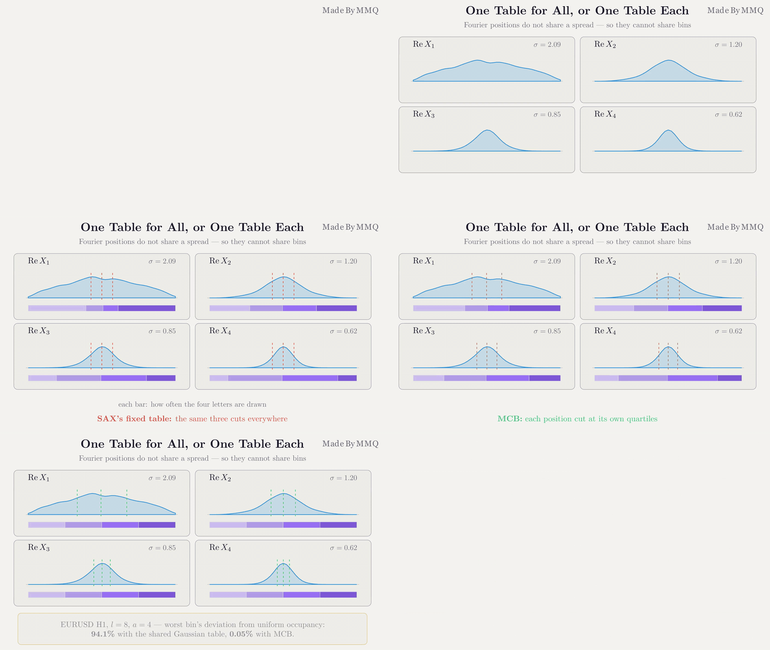
Fig. 3. Value distributions for four coefficient positions, with the shared Gaussian cuts and the fitted MCB cuts drawn over them
The Lower Bound and Its Factor of Two
A symbolic representation is only useful for search if the distance between two words lower-bounds the true distance between the underlying windows. That property is what lets a search reject a candidate without ever computing its real distance, and reject it soundly, with a guarantee that no genuine match was thrown away.
The per-position argument is the one SAX uses: equal or adjacent bins contribute nothing, since values either side of a shared edge can sit arbitrarily close, and anything further apart is separated by at least the gap between the edges it straddles.
//+------------------------------------------------------------------+
//| Distance between two symbol codes at position j.                 |
//|                                                                  |
//|  Equal or adjacent bins contribute nothing, because two values in|
//|  neighboring bins can sit arbitrarily close on either side of    |
//|  their shared edge. Otherwise the values are separated by at     |
//|  least the gap between the outer edges they straddle.            |
//+------------------------------------------------------------------+
double CSFATransform::CellDist(int j,int c1,int c2) const
  {
   if(!m_fitted || j<0 || j>=m_word)
      return 0.0;

   int hi=(c1>c2)?c1:c2;
   int lo=(c1<c2)?c1:c2;
   if(hi-lo<=1)
      return 0.0;

   int    base=j*(m_a-1);
   double gap=m_beta[base+hi-1]-m_beta[base+lo];
   return (gap>0.0)?gap:0.0;
  }
The interesting part is converting a bound in coefficient space into a bound on the original series. Parseval gives the conversion, but with a subtlety that is easy to get wrong and expensive to get wrong silently. A real-valued signal has a conjugate-symmetric spectrum: coefficients k and n-k have identical magnitude, so summed over the full spectrum every retained coefficient counts twice. The bound can therefore legitimately carry a factor of two, which makes it meaningfully tighter than the naive version. The catch is that the Nyquist bin at k = n/2 is its own mirror, which is why configuration refuses word lengths that would reach it.
//+------------------------------------------------------------------+
//| Lower bound on the true Euclidean distance, from words alone.    |
//|                                                                  |
//|  The chain has two links. Per position, the quantization argument|
//|  gives |dValue_j| >= CellDist_j, so the retained coefficients    |
//|  differ by at least sum(CellDist^2). Parseval then converts that |
//|  into a bound on the original series — and because a real signal |
//|  has conjugate-symmetric spectrum, every retained coefficient k  |
//|  is mirrored at n-k and counts twice. Hence the factor 2, which  |
//|  is exactly why Configure() refuses word lengths that would reach|
//|  the unmirrored Nyquist bin.                                     |
//|                                                                  |
//|  MinDist <= ApproxDist <= TrueDist holds for every pair; the     |
//|  validation script asserts that ladder directly. Returns -1 on a |
//|  length mismatch.                                                |
//+------------------------------------------------------------------+
double CSFATransform::MinDist(const int &wordA[],const int &wordB[]) const
  {
   if(!m_fitted)
      return -1.0;
   if(ArraySize(wordA)!=m_word || ArraySize(wordB)!=m_word)
      return -1.0;

   double sum=0.0;
   for(int j=0;j<m_word;j++)
     {
      double d=CellDist(j,wordA[j],wordB[j]);
      sum+=d*d;
     }
   return MathSqrt(2.0*sum);
  }
This gives a three-rung ladder, each rung measuring the cost of a different approximation:
MinDist <= ApproxDist <= TrueDist
MinDist works from the letters alone. ApproxDist works from the unquantized coefficient vectors, so the step between the two is exactly what quantization costs. TrueDist is the full-length Euclidean distance between the z-normalized windows, so the step up to it is exactly what discarding the high-frequency coefficients costs. Only the outer inequality matters for search, but checking both localizes a break: a broken cell table snaps the left rung, a broken basis or a wrong factor of two the right one.
Both bounds carry a constant factor that puts them on the axis of the true distance, and the two are the same kind of bookkeeping: SAX's MINDIST multiplies by sqrt(n/w) because each PAA mean stands in for n/w bars, SFA's by sqrt(2) because each stored coefficient stands in for itself and its mirror. Neither is an empirical fudge. What differs is where the normalization lives: SFA folds 1/sqrt(n) into its basis, so only the mirror count remains.
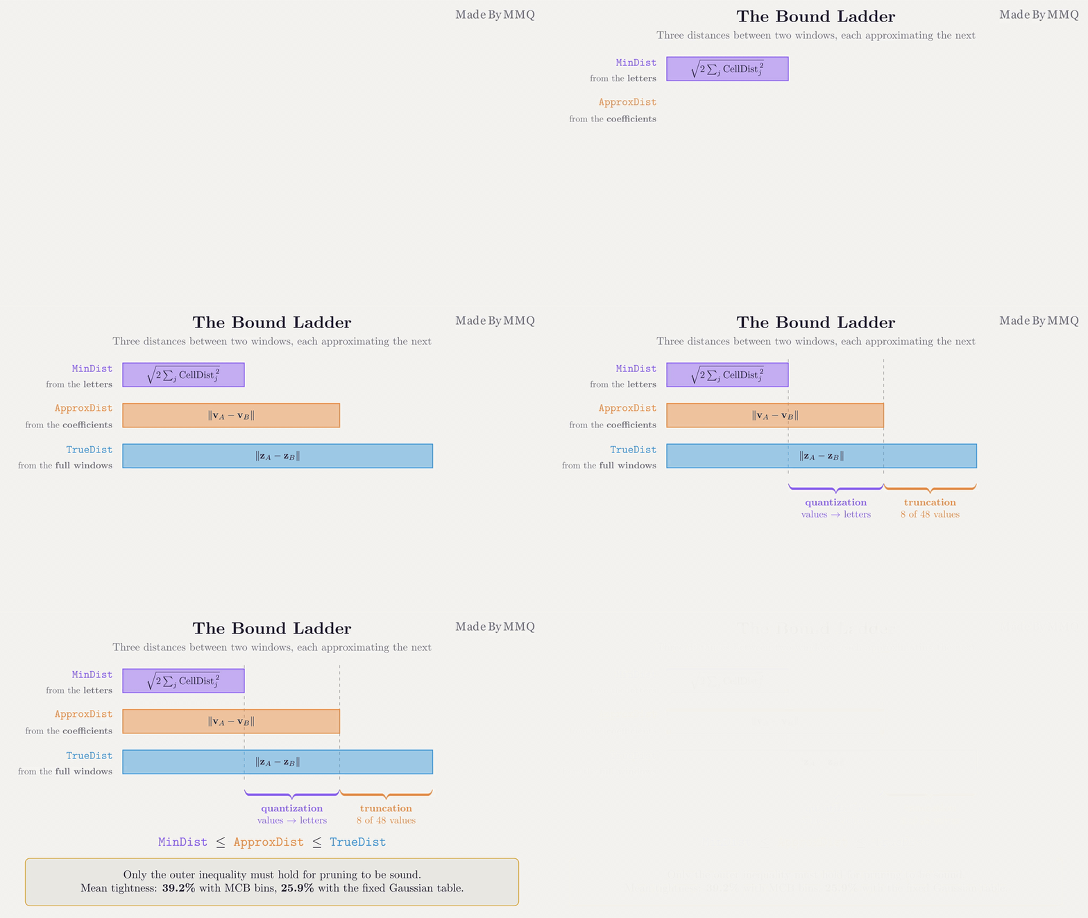
Fig. 4. The bound ladder: quantization separates the first two rungs, coefficient truncation separates the last two
From Words to Precedents
With a sound bound in hand, the search answers the practical question: the current window looks like this, when has it looked like this before, and what happened next?
The design rule is that the symbolic word never decides the ordering; it exists only to reject candidates cheaply. Everything that survives is ranked by the true full-length Euclidean distance between z-normalized windows. This costs a little more per surviving candidate, and it buys the guarantee that the two-stage pipeline returns exactly what an exhaustive scan would return, which the validation script checks directly.
Two guards keep the output honest, and the second one is new relative to SAX.
No lookahead. A candidate's outcome window must close strictly before the query window opens: if a match ends at bar cEnd and we read its next H bars, then cEnd + H must fall before the query's first bar. This is the ordinary guard any historical-analog tool needs.
No bin leakage. This one is specific to SFA, and it exists precisely because MCB learns from data. SAX's breakpoints are constants that never touch the price series, but our bin edges do, so a careless fit over all history would let the query window, and everything after it, influence how letters are drawn. The fix is to fix the candidate region first and confine the fit to it, so that every window shaping the edges is one the search was already permitted to see.
//--- latest candidate end that keeps the whole outcome window in the past
   int lastEnd=qStart-H-1;
   if(lastEnd<L-1)
      return false;                  // not enough history for any analog

//--- fit the MCB edges once, over the candidate region only
   if(!m_sfa.IsFitted())
     {
      int span=lastEnd-(L-1)+1;
      int stride=m_fit_stride;
      if(stride<1)
         stride=(int)MathMax(1.0,MathCeil((double)span/(double)SFA_FIT_TARGET));
      if(!m_sfa.FitFromSeries(close,n,L-1,lastEnd,stride))
         return false;
      m_fit_windows=m_sfa.FitCount();
     }
That is an excerpt from the middle of Find; the surrounding function sets up the query window and then runs the scan. The pruning stage is where the bound earns its place:
      double md=0.0;                 // lower bound (stays 0 when unused)

      //--- stage 1: reject on the bound alone
      if(m_metric==SFA_METRIC_MINDIST)
        {
         int cword[];
         if(m_sfa.Encode(craw,L,cword)!=SFA_OK)
            continue;                // flat candidate
         md=m_sfa.MinDist(m_query_word,cword);
         if(md<0.0)
            continue;
         if(m_found>=m_max_analogs && md>=m_analogs[m_found-1].distance)
           {
            m_pruned++;
            continue;
           }
        }
Once the result buffer is full, a candidate whose lower bound meets or exceeds the worst distance held cannot enter the top-k, so its true distance is never computed. This is a sequential scan with a filter in front of it, not an index: every candidate is visited, and the bound decides which get a true distance. SFA_METRIC_EUCLID skips the bound and measures every candidate, producing identical rankings, which makes it both a correctness and a speed baseline.
Outcomes are expressed in multiples of the ATR at the time of the match, so precedents from calm and violent regimes sit on a comparable footing. The collection of those forward moves, not any single prediction, is the product of the tool.
Verifying It Works
SFAValidate.mq5 runs twenty checks. They are worth walking through not as a list but as a sequence of questions, because each one is designed to catch a specific class of error that would otherwise leave every later number quietly wrong.
Is the transform actually a DFT? The first test evaluates the retained coefficients by direct summation, independently of the cached basis, and compares term by term. This catches a sign error on the imaginary part or an off-by-one in the coefficient index, either of which would leave every subsequent test passing on consistently wrong numbers. Maximum absolute difference: 1.776e-15.
Does energy land where it should? A pure cosine at frequency 3 over 48 bars must put all its energy into the real part of coefficient 3 and leave every other retained value at zero. Under our scaling that value is sqrt(n/2) = 4.898979. The sqrt(2) is easy to lose: a unit cosine has a standard deviation of 1/sqrt(2), so z-normalization scales it up before the transform sees it, and working the number out without that step gives sqrt(n)/2 instead. Measured: 4.898979, with maximum leakage elsewhere of 3.469e-15. This single test confirms the basis, the indexing, and the normalization at once.
Is the factor of two right? This is the test that would be most painful to omit, because a wrong factor of two produces a bound that is still monotone, still plausible, and still wrong. The trick is to choose a window length where no coefficient is discarded, so the inequality collapses into an equality. The excerpt below is the setup; the loop that follows compares 200 random pairs.
//+------------------------------------------------------------------+
//| Test 3: Parseval. When no coefficient is discarded the           |
//| approximation distance must EQUAL the true Euclidean distance,   |
//| not merely bound it — the scaled DFT is an isometry.             |
//|                                                                  |
//|  An odd window length is used deliberately: with n odd there is  |
//|  no unpaired Nyquist bin, so retaining k=1..(n-1)/2 accounts for |
//|  the entire spectrum once the zero DC term is set aside. Any     |
//|  error in the factor 2 shows up here as a fixed ratio, not noise.|
//+------------------------------------------------------------------+
void TestParsevalExact()
  {
   int n=49;                       // odd: no Nyquist bin to leave behind
   int l=n-1;                      // every non-DC coefficient retained
   CSFATransform sfa;
   Check("configure full-spectrum n=49 l=48",
         sfa.Configure(n,l,4,SFA_BINS_GAUSSIAN),"");
Maximum relative error over 200 trials: 8.434e-16, which is the accumulated rounding of the sums and nothing else. Halve or double the factor and this number becomes 0.29 or 0.41 instead, the same on every trial.
Does the ladder hold? Three thousand window pairs, each rung checked separately, in all three binning modes, because all three must produce a valid bound. They differ in tightness, never in soundness. The windows are synthetic random walks rather than price data, deliberately: the bound is a mathematical claim about any input, so the test that checks it should not be able to pass by getting lucky on one instrument. Result: 0 violations out of 3000 in every mode. The same test reports tightness as a byproduct, and this is where the ablation shows up.
| Binning mode | Bound tightness |
|---|---|
| Equi-depth (MCB) | 39.2% |
| Equi-width | 35.1% |
| Fixed Gaussian | 25.9% |
Tightness is the mean of bound divided by true distance, so higher is better: 100% would be exact, and 0% would never reject anything. All three rows use l = 8, a = 4 and the same 3000 pairs, so the only thing that changes between rows is the bin table. The ordering confirms that the Fourier front end alone is not the story: swapping MCB for the fixed Gaussian table costs roughly a third of the bound's strength while changing nothing else.
Does the search behave? The final group runs on live history and checks four conditions at once: no lookahead, an MCB fit confined to the candidate region, two-stage results bit-identical to brute force, and pruning that actually happened. The newest analog ends at bar 5929 against a latest permitted bar of 5939, the fit uses 2947 windows against a structural ceiling of 2947, and the two-stage result matches brute force with a maximum distance difference of 0.0e+00, meaning identical and not merely close.
SAX vs SFA on Identical Windows
SFACompare.mq5 is the reason this article exists. It encodes the same windows under several codings, each spending w letters over an alphabet of a and each bounding the same distance, so the comparison is like for like. Because SFA changes both the front end and the bin table, the script adds a control, PAA-MCB: SAX's PAA cells cut at learned per-position quantiles. SAX to PAA-MCB changes only the table; PAA-MCB to SFA changes only the front end. SAXTransform.mqh from the previous article is attached so the download compiles as it stands.
The learned bins are fitted on one part of the history and everything is measured on another: by default the older and newer halves, while InpSplit reverses them or fits on only the oldest quarter to age the bins on purpose. SAX needs no split, since its breakpoints are constants. Unless stated otherwise, every run loads 12000 bars ending 10 August 2026 at 12:00, pinned by InpEndTime so the numbers reproduce.
Are the bounds sound, and how tight are they? Across roughly 20000 random window pairs, none of the three codings produced a single lower-bound violation. SFA's bound is the tightest in all nine runs, the seven EURUSD H1 configurations below plus GBPUSD H1 and EURUSD H4: at w = 8, a = 8 it averages 60.5% of the true distance against 58.6% for PAA-MCB and 56.7% for SAX. It is also far less often degenerate, exactly zero and so unable to reject anything: 0.12% of pairs against SAX's 1.23%.
How much work does each bound save? Pruning depends on the running threshold, which depends on scan order. The harness drives the scan with the true distance and counts, for each candidate, what each bound would have said at that exact threshold, a clean counterfactual with no order dependence. It counts avoided true-distance computations, not wall-clock time: encoding, fitting and data access are outside the count.
         //--- what each bound would have said, at this exact threshold
         int sw[],pw[],fw[];
         ArrayResize(sw,InpWordLen);
         ArrayResize(pw,InpWordLen);
         ArrayResize(fw,InpWordLen);
         for(int j=0;j<InpWordLen;j++)
           {
            sw[j]=g_saxWords[c*InpWordLen+j];
            pw[j]=g_pmWords[c*InpWordLen+j];
            fw[j]=g_sfaWords[c*InpWordLen+j];
           }
         if(g_sax.MinDist(qsax,sw,L)>=thr)
            saxPrune++;
         if(g_pm.MinDist(qpm,pw)>=thr)
            pmPrune++;
         if(g_sfa.MinDist(qsfa,fw)>=thr)
            sfaPrune++;
How many true neighbors does each recover? This is where the codings part company. Ranking purely by symbolic distance is the approximate search you would run on a history too large to scan exactly. Recall is the overlap between that ranking's top 50 and the exact top 50 on the clean query, with windows overlapping the query excluded from both, since they are the query shifted by a few bars. It measures how faithfully the letters preserve neighborhoods, not what those neighbors predict; the indicator re-ranks every survivor by true distance, so its output equals an exhaustive scan whatever the recall.
The harness averages over 120 queries one window apart, covering the whole measured half. Every coding answers the same queries, so each gap is measured query by query and reported with its paired standard error; a gap beyond about twice its standard error is one the query sample cannot explain away. Here is the sweep on EURUSD H1, sorted by how the budget was split, with Bits as w · log2(a) rounded up:
| Word length w | Alphabet a | Bits | SAX recall % | PAA-MCB recall % | SFA recall % | SFA - SAX (se) |
|---|---|---|---|---|---|---|
| 6 | 10 | 20 | 29.2 | 32.8 | 39.6 | +10.4 (1.5) |
| 8 | 10 | 27 | 39.1 | 45.7 | 47.2 | +8.1 (1.4) |
| 8 | 8 | 24 | 34.0 | 39.0 | 44.2 | +10.2 (1.6) |
| 10 | 10 | 34 | 49.2 | 50.6 | 52.8 | +3.6 (1.1) |
| 8 | 4 | 16 | 10.6 | 9.0 | 13.8 | +3.3 (1.0) |
| 24 | 6 | 63 | 46.8 | 50.2 | 46.6 | -0.2 (1.4) |
| 16 | 4 | 32 | 20.8 | 20.5 | 21.1 | +0.3 (1.4) |
SFA's lead is large where the alphabet is deep and the word short: 8 to 10 points at a = 8 or 10 with six or eight positions, six to seven standard errors. With a = 10 it shrinks as positions are added, from 10.4 at w = 6 to 8.1 at w = 8 and 3.6 at w = 10, and at 16 or 24 positions it is gone, well inside the standard error. SAX comes out ahead nowhere; at the shallow, wide end the two tie. The mechanism is plausible.
SFA wants depth. Its information sits in the few lowest frequencies. A deep alphabet resolves those positions finely; spending the budget on more positions buys high-frequency coefficients with little signal, which is what happens at w = 16 and 24.
SAX wants breadth. After z-normalization every PAA cell has roughly the same variance, so information is spread evenly. More cells help it, and at 24 cells PAA with learned bins is the strongest coding in the table.
PAA-MCB splits SFA's lead into its sources. At w = 8, a = 8 the learned bins alone add 4.9 points (standard error 1.1) and the Fourier front end another 5.3 (1.3), roughly half each. The balance moves: at w = 8, a = 10 it is mostly the table (6.6 against 1.5), at w = 6, a = 10 mostly the transform (6.8 against 3.6), and at w = 24, a = 6 the transform works against SFA, with PAA-MCB ahead by 3.5 (1.3). With many positions, PAA is the better front end once it gets learned bins.
The efficiency consequence is the practical headline: SFA at 27 bits scores 47.2 against SAX's 46.8 at 63 bits, and SFA at 20 bits 39.6 against SAX's 39.1 at 27. Configured to its strength, SFA reaches SAX-class recall on less than half the budget. Those are per-word bits; SFA's learned table, w · (a-1) edges or 4608 bits at w = 8, a = 10, adds under a bit per word spread over the 6000 measured windows, while SAX's breakpoints are constants.
That does not make the method matter more than the configuration. SAX at 34 bits with ten letters scores 49.2, SFA at 32 bits with four letters 21.1: set the alphabet first, whichever coding you use.
Pruning follows tightness at deep alphabets, 57.4% of candidates against SAX's 54.1% at w = 6, a = 10, but at a = 4 the two are level (30.4% against 30.5% at w = 8), so a tighter average bound does not always buy more pruning.
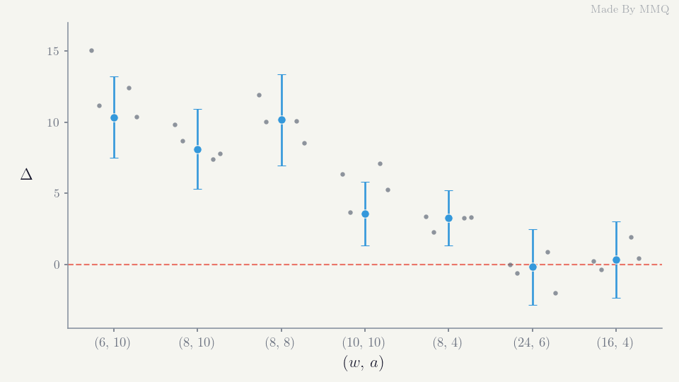
Fig. 5. SFA recall minus SAX recall for each (w, a): blue is the main run with a 95% interval, grey the four robustness runs; the dashed line is no difference
Fig. 5 adds four more runs of each configuration: the split reversed, a stale fit on the oldest quarter, and two earlier two-year periods ending August 2024 and August 2022. The pattern holds in every one: at a = 8 or 10 the lead ranges from 3.6 to 15.1 points, always significant; at (8, 4) from 2.3 to 3.4; at (24, 6) and (16, 4) from -2.0 to +1.9, inside the noise. Bin aging, the obvious worry with a learned table, cost nothing measurable: the stale fit gave +10.1 at w = 8, a = 8 against +10.2 with fresh bins.
Nor is the lead an artifact of one market. At w = 8, a = 8:
| Market | SAX recall % | PAA-MCB recall % | SFA recall % | SFA - SAX (se) |
|---|---|---|---|---|
| EURUSD H1 | 34.0 | 39.0 | 44.2 | +10.2 (1.6) |
| GBPUSD H1 | 33.9 | 37.7 | 42.6 | +8.7 (1.5) |
| EURUSD H4 | 34.8 | 39.8 | 43.0 | +8.2 (1.6) |
What about noise? The harness also measures symbol flip rate: how many letters change when a window is re-encoded after a calibrated disturbance. SFA flips more than SAX at every noise level in every configuration; at w = 8, a = 8, 5.5% against 3.3% under the mildest disturbance and 37.4% against 27.1% under the harshest. The obvious explanation, that SAX under-uses its alphabet and so rarely crosses a bin edge, fails against the control: SAX's letter entropy is already 0.966 of the maximum, and PAA-MCB, as even as SFA at 0.998, flips almost as rarely as SAX (3.6% and 29.4%). The difference is the front end. A PAA cell averages six bars, cutting the noise reaching each letter by roughly the square root of six, while SFA's quiet high-frequency positions have narrow learned bins that noise crosses easily. Whether the extra flips matter shows in retrieval:
| Noise level | SAX recall % | PAA-MCB recall % | SFA recall % | SFA - SAX (se) |
|---|---|---|---|---|
| clean | 34.0 | 39.0 | 44.2 | +10.2 (1.6) |
| 0.05 | 34.3 | 38.8 | 44.1 | +9.8 (1.6) |
| 0.10 | 33.9 | 38.4 | 43.7 | +9.8 (1.6) |
| 0.20 | 33.3 | 38.5 | 42.2 | +8.9 (1.6) |
| 0.40 | 30.4 | 33.0 | 37.6 | +7.2 (1.4) |
Noise is scaled to each query window's own standard deviation, and the target is always the exact top 50 of the clean query, so a falling column means real neighbors were lost. SFA still recovers more at every level, but the extra flips are not free: it gives up 6.6 points from clean to the harshest noise against SAX's 3.6, and its lead narrows from 10.2 to 7.2. It stays ahead because it starts far ahead, not because it is more robust. Symbol stability and retrieval quality are different properties, and a representation should be judged on the second.
The Indicator
SFAAnalog.mq5 puts the search on a chart. It draws two things: a fan cone over the next H bars, and a corner panel carrying the verdict and the diagnostics.
The cone is not a forecast line, and the distinction matters. At each forward step it plots the median and the 25th to 75th percentile band of what actually happened after the closest historical matches, scaled by the current ATR so it sits on the real price axis. A wide band means the precedents disagreed, which is itself the useful signal.
It is also drawn only when the sample earns it, which is worth stating in numbers rather than leaving to the phrase "high conviction". Three gates stand between a set of analogs and a direction on the chart, and a sample must clear all of them.
//+------------------------------------------------------------------+
//| Turn the stats into a verdict.                                   |
//|  Order matters: too-few analogs is decided first, then the       |
//|  coin-flip case, and only a sample clearing BOTH the median-move |
//|  and up-rate bands earns a direction.                            |
//+------------------------------------------------------------------+
void CSFAAnalogFinder::Classify(void)
  {
   if(m_found<m_min_analogs)
     {
      m_stats.verdict=SFA_ANALOG_TOO_FEW;
      return;
     }

   double med=m_stats.median_atr;
   double up =m_stats.up_rate;

   bool weakMove=(MathAbs(med)<m_edge_atr);
   bool weakDir =(up<m_min_uprate && up>1.0-m_min_uprate);
   if(weakMove || weakDir)
     {
      m_stats.verdict=SFA_ANALOG_NO_EDGE;
      return;
     }

   m_stats.verdict=(med>0.0)?SFA_ANALOG_BULLISH:SFA_ANALOG_BEARISH;
  }
At the defaults that means at least 10 analogs, a median forward move of at least 0.25 ATR in absolute value, and an up-rate outside the band from 42% to 58%. Fail any one and the verdict is no edge or too few analogs, the chip turns grey and no cone is drawn. An empty chart is therefore a verdict rather than a failure, and it is the common case: on most bars the precedents genuinely disagree.
The panel carries two rows the SAX version cannot: the size of the MCB fitting sample, and the share of candidates the lower bound rejected on this bar. The first tells you whether the bin edges rest on enough history to mean anything; the second tells you what the symbolic layer is actually buying. Labels sit flush left and values are anchored by their right edge, which keeps the columns true without a monospace font; only the symbolic word is monospaced, because there the letters themselves carry meaning.
One operational detail the panel exists to expose. The MCB edges are fitted on the first call and then reused, because refitting on every bar costs a full history pass to move edges that barely drift. The MCB BINS row is how you audit that: the fit caps its sample near four thousand windows, so a figure in the thousands is healthy, while one in the low hundreds means the chart does not carry enough history for the bins to mean much. Over a long live run the edges will age; reload the indicator, or call ResetFit on a schedule of your own choosing. The stale-fit run suggests the aging is slow, but SAX has no equivalent concern at all, and that is a real cost of learning the bins rather than assuming them.
| Input | Default | What it controls |
|---|---|---|
| InpWinLen | 48 | Shape window in bars, the n of the transform |
| InpHorizon | 12 | Forecast horizon H, and the width of the cone |
| InpWordLen | 8 | Word length, must be even and clear of the Nyquist bin |
| InpAlphabet | 8 | Alphabet size, 2 to 10. The parameter the sweep is about |
| InpBinning | EQUI_DEPTH | Bin rule; the other two modes are there for comparison |
| InpMinAnalogs | 10 | Sample below which the verdict is too few analogs |
| InpEdgeATR | 0.25 | Median move, in ATR, needed to count as a lean |
| InpMetric | MINDIST | Two-stage search, or EUCLID to measure every candidate |
| InpMaxHistory | 6000 | Bars scanned for precedents, and fitted for the bins |
The default configuration is w = 8 with a = 8, not the a = 4 that would mirror a typical SAX setup. That is a deliberate consequence of the measurements: at a = 4 SFA's lead shrinks to a few points or disappears, so shipping that default would throw away the representation's main strength.
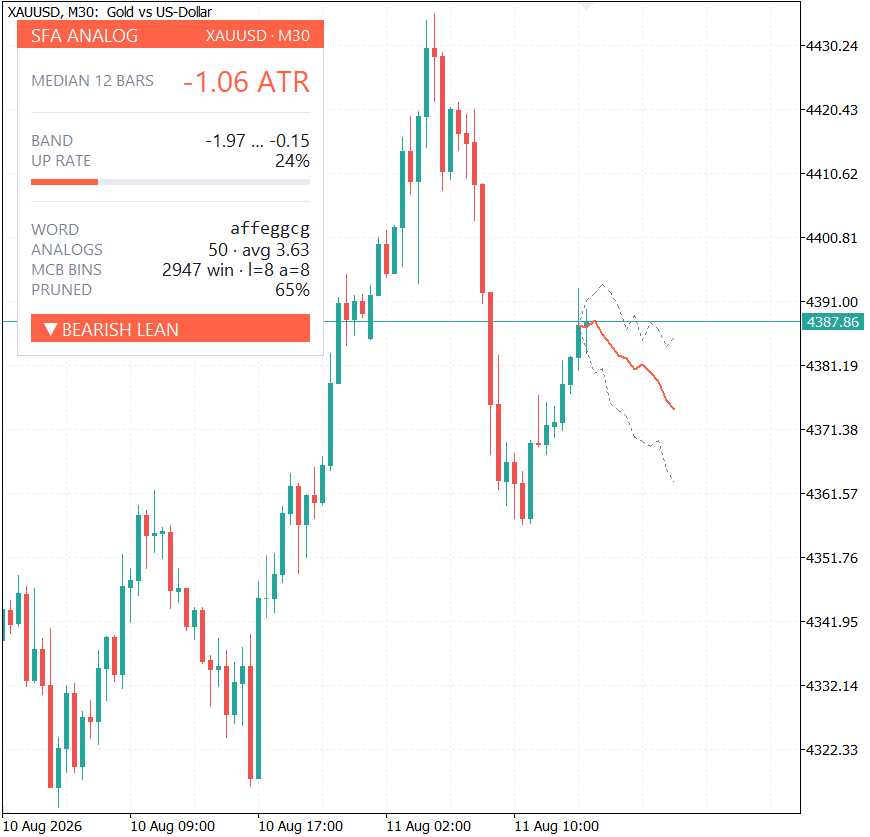
Fig. 6. The indicator on XAUUSD M30: hero row, up-rate bar, diagnostics, and the verdict chip
Conclusion
We set out to answer whether the Fourier domain earns its place in a symbolic similarity search. It does, by a wide margin where the bit budget buys a deep alphabet, and by nothing where the budget is spread over many shallow positions, a more useful answer than a blanket win because it tells you how to configure the method.
- Spend SFA's budget on depth, not breadth. With six or eight letters over an alphabet of 8 or 10, SFA beat SAX by 8 to 10 recall points at six to seven standard errors; with 16 or 24 letters over 4 or 6, the two tied. SAX came out ahead in no configuration, across three fit/measure splits and three two-year periods.
- SFA is the more efficient representation when configured to its strength. Twenty-seven bits of SFA scored 47.2 against SAX's 46.8 at sixty-three, and twenty bits matched SAX at twenty-seven, with the learned table adding under a bit per word. Configuration still matters more than method: SAX at thirty-four bits with ten letters scores 49.2, SFA at thirty-two bits with four letters 21.1. Set the alphabet first.
- The learned bins supply about half of the recall lead. At w = 8, a = 8 they add 4.9 points to SAX's own PAA cells, and the Fourier front end 5.3 more; at w = 24, PAA with learned bins beats SFA by 3.5. The price is a fitting pass, a stored table, and edges that age, though a fit six months stale lost no measurable recall.
- The bound was tighter in every run, and MCB is why. SFA's bound was the tightest of the three codings in all nine runs and far less often degenerate, and swapping MCB for the fixed Gaussian table costs a third of its tightness. But a tighter bound is a pruning property, not a ranking one: at (16, 4) it is three points tighter while recall ties, and at a = 4 it buys no extra pruning.
- Do not judge a symbolic representation by symbol stability. At w = 8, a = 8, SFA flips 1.4 to 1.7 times as many letters as SAX under noise while retrieving more true neighbors at every level. The flips come from the front end, not alphabet use: PAA averages noise before it reaches a letter, which is why PAA with learned bins flips almost as rarely as SAX.
The most transferable part of this work is the harness. Bound tightness, degenerate-bound rate, pruning power, and neighbor recall are four cheap numbers that tell you whether any symbolic representation is spending your bits well, on your symbol, at your settings; adding a coding means implementing an encoder and a distance. To use it, open SFACompare.mq5 on your chart, sweep InpAlphabet first, and read the recall gap with its standard error. If SFA leads at your budget, the indicator's defaults already sit in the right regime.
The scope deserves stating plainly. The full sweep ran on EURUSD H1; GBPUSD H1 and EURUSD H4 were checked at one configuration, and walk-forward refitting was not tested. The 48-bar window is short by the standards of the literature, where 128 to 1024 is typical, so aggressive compression of long windows, where Fourier energy compaction should matter most, remains untested. And the depth-over-breadth result is a direct prediction for bag-of-words classification: the BOSS ensemble holds the alphabet at four, the corner where SFA's lead was smallest here, so rerunning it with a deeper alphabet is a cheap experiment with a testable outcome.
Getting the Source Code via MQL5 Algo Forge
All source files are attached to this article below, but the full repository is also available on MQL5 Algo Forge, the community's Git-based platform for sharing and collaborating on trading projects.
| File name | Description |
|---|---|
| MQL5\Include\SFA\SFATransform.mqh | SFA core transform: truncated DFT front end, MCB bin fitting in three modes, per-position cell table, and the lower bound |
| MQL5\Include\SFA\SFAAnalogs.mqh | Historical analog search ranked by true Euclidean distance and pruned by the SFA bound, with no-lookahead and no-bin-leakage guards |
| MQL5\Scripts\SFA\SFAValidate.mq5 | Twenty-check validation harness: DFT correctness, Parseval exactness, the bound ladder in all binning modes, and live-search equivalence to brute force |
| MQL5\Scripts\SFA\SFACompare.mq5 | SAX versus SFA on identical windows, with a PAA-MCB control: bound soundness and tightness, pruning power, symbol flip rate and letter entropy under noise, and true-neighbor recall with paired standard errors |
| MQL5\Include\SAX\SAXTransform.mqh | The SAX transform from the previous article, carried over unmodified in behavior. Included by SFACompare.mq5 and attached so the comparison compiles as downloaded |
| MQL5\Indicators\SFA\SFAAnalog.mq5 | Chart indicator drawing the forward fan cone and the verdict panel |
Warning: All rights to these materials are reserved by MetaQuotes Ltd. Copying or reprinting of these materials in whole or in part is prohibited.
This article was written by a user of the site and reflects their personal views. MetaQuotes Ltd is not responsible for the accuracy of the information presented, nor for any consequences resulting from the use of the solutions, strategies or recommendations described.

 State Persistence in MQL5 (Part 1): A Crash-Safe State Store That Survives a Restart
 Uncertainty as a Model (Part 2): Dependence Among Random Variables — From Correlation to Copulas
 Building a Divergence System (Part IV): Creating a Reusable Divergence Engine for MQL5
 Building Volatility Models in MQL5: Implementing the APARCH Volatility Process

- Free trading apps
- Over 8,000 signals for copying
- Economic news for exploring financial markets
You agree to website policy and terms of use