Defining your Edge (Part 6): Harnessing Fourier Transform and a Spiking Neural Network in an Expert Advisor

Introduction

We resume our series on Defining your Edge in the markets by introducing a variant to the article-format we have presented so far. In the first five parts we introduced algorithm and network pairings. That article-format was about discovering and testing novel algorithms and neural-networks that are not mainstream; for this article we are "doing the opposite" of this exploration by looking at how to possibly exploit algorithm and neural-network pairings that have already been introduced.

Therefore, this 6th part, returns to the algorithm-network pairing that started this series. This earlier article united a Discrete Fourier Transform with a small Leaky Integrate-and-Fire Spiking Neural Network. The Fourier computation searched price, MACD and RSI for recurring structure. The Neural Network served as an extra layer that let directional stimulation (or votes) accumulate across completed bars before a signal was launched.

This time we want to examine in what way the same EA behaves when its seven operating modes are applied to different settings. This could be taken as a key step in the adoption and use of this model although there are different approaches to our own that could be taken to accomplish the same result. In our testing reports presented below, we change up the symbol, timeframe, and test-window. The symbol EURUSD is used twice due to its liquidity but again this method is not cast in stone as the reader can always change things up.

Every report presented below is a forward-run check. On average, two thirds of the test window supplied the optimization sample with the final third staying reserved for the forward walk. The chosen inputs are then run through this later, one-third segment without any extra adjustments, as a forward walk. From the testing reports, five were able to finish profitably while two were in the red. Both of these are discussed below, since we take the loss to mark where our input settings could be unfit which could be more pragmatic than picking another symbol or test window where we get "good results".

Seven checks could not settle the argument if this model has a durable edge. They only offer practical leads. Continuous rolling-windows, harsher costs, frozen parameters and a wider regime coverage are all aspects the reader needs to consider first before considering live use. Our task though, is to spot which local settings deserve more work.

Recap on the Fourier and SNN

We introduced the algo-network pairing in this article. In it we made the case how the Fourier and SNN components deal with alternative parts of the Signal problem. The Fourier computation shows a finite market sequence through frequency components. Given a rolling array x[n] with length N, the DFT gives us complex coefficients X[k]. The real and imaginary portions of these coefficients describe amplitude and phase. The Trade Robot skips the zero-frequency component, by searching up to the Nyquist limit and then chooses the greatest amplitude. A sine projection converts this phase into a score between -1 and 1.

The score does not show a permanent cycle or give us a statistical forecast. The calculation simply describes the period component that is strongest within the current window. An alternative frequency could take the lead as bars join and leave the array buffer. 'InpFourierWindow' therefore controls the observation horizon. A shorter buffer-window could react too quickly causing one to chase noise. A longer one is bound to retain the old structure even after the market has evolved.

A key turning threshold adjudicates when the Fourier score becomes directional. Readings that are close to zero would get ignored. Positive and negative extremes are meant to support buy and sell signals. For our algorithm, modes 0, 1, and 2 all apply the same spectral search to closing price, the MACD main line as well as RSI. The SNN adds state through a compact Leaky Integrate-and-Fire design. Separate bullish and bearish membrane potentials hold weighted stimulation. On every completed bar, the input 'InpSnnDecay' omits part of the kept charge before new evidence can be added. When one potential gets to the 'InpSnnThreshold', the neuron returns a direction and we reset.

Decay and threshold determine the response together. Heavy decay can forget simulation quickly, while a low threshold would require less accumulated evidence. Low decay keeps more history. A high threshold requires more bars to be in agreement. Their effect is subject to input scale and persistence. Our Trade-Robot's enumerations are meant to map to a separate operation mode for the algorithm. This separation helps expose every route. A price-spectrum mode could be suited on one chart, while a slowly sampled indicator-pattern SNN could struggle elsewhere. Our reports below examine these local fits without treating the hybrid as one indivisible signal.

Exploiting the Modes

The seven modes make up separate signal paths. Mode-0 transforms closing prices; Mode-1 changes MACD values; while Mode-2 deals with the RSI. Mode-3 sends combined spectral information through the SNN. Mode-4 engages price action, Mode-5 relies on indicator patterns, while the final mode, Mode-6 brings together Fourier phase, RSI and MACD momentum.

Testing all these routes on GBPJPY on the 2-hour timeframe would just answer one narrow question. In this implementation though, all the modes get a different symbol, timeframe, and calendar test window. The slower 6-hour and 8-hour timeframes use-cases are tested with wider test windows. On the flip side the 15-minute and 30-minute timeframe tests get smaller test windows given the number of data points and therefore higher compute costs. This approach though is flawed in that the length of the test window (with longer windows being better) is the only critical component in verifying a model. A lot of data points, and thus a lot of trades could actually amount to white noise, IMHO. That said, our end output from these tests is not a ranking on which mode is best but rather a deployment probe on how our model actually works.

All reports begin with USD 10,000,  1:100 leverage and 0.10 lots. The MACD oscillator is used with its typical periods of 12, 26, and 9 while the RSI period also remains pegged at 14. The history quality we use seems decent clocking in at almost 100%. Every local optimization gives us the Fourier window, turning threshold, SNN settings and execution deviation.

Our used MetaTrader forward fraction is one-third of the test window. For instance if the EURUSD 1-hour test spans from September 2023 to September 2026, then the first two years are used to optimize with the final year applied to the forward walk. Other modes with different symbols and timeframes use a similar proportion for optimization and a forward walk. The chosen parameter set is judged only on its own reserved segment.

In this analysis, several axes change concurrently, so a larger profit cannot be attributed only to one test mode. Net profit indicates if the account advanced while the Profit Factor compares gross profit with the gross loss. Equity drawdown logs the deepest mark-to-market drop while Recovery Factor compares the Profit Factor to this decline. The other key metrics could be Sharpe Ratio that describes return consistency while trade count logs how busy the model was during testing. As argued already, we do not have a universal pass mark per se. A modest gain could warrant an extra test. A loss with just twenty trades could not be as definitive, as one with two hundred; nonetheless neither result warrants a test mode to be ruled out. Our goal here can be seen as narrowing the research for the next phase.

To recap from the referenced article, mode selection is implemented as follows in MQL5:

//+------------------------------------------------------------------+
//| Expert tick function                                             |
//| Description: Coordinates state changes and signal routing to open|
//|              or close trades on the completion of each bar.      |
//+------------------------------------------------------------------+
//+------------------------------------------------------------------+
//| Expert tick function                                             |
//+------------------------------------------------------------------+
void OnTick()
  {
//--- Execute only on a new bar
   datetime timeCurrentBar = iTime(_Symbol, _Period, 0);
   if(timeCurrentBar == timeLastBar)
      return;
   int signal = 0; // 0 = No signal, 1 = Buy, -1 = Sell
//--- Route execution to the selected function mode
   switch(InpMode)
     {
      case MODE_FOURIER_PRICE:
         signal = ExecuteFourierPrice();
         break;
      case MODE_FOURIER_MACD:
         signal = ExecuteFourierMACD();
         break;
      case MODE_FOURIER_RSI:
         signal = ExecuteFourierRSI();
         break;
      case MODE_FOURIER_COMBINED:
         signal = ExecuteFourierCombined();
         break;
      case MODE_PRICE_ACTION_SNN:
         signal = ExecutePriceActionSNN();
         break;
      case MODE_INDICATOR_PATTERN:
         signal = ExecuteIndicatorPatternSNN();
         break;
      case MODE_HYBRID_FULL:
         signal = ExecuteHybridFull();
         break;
     }
//--- Process Trading Signals
   if(signal != 0)
     {
      ManagePositions(signal);
      timeLastBar = timeCurrentBar;
     }
  }

Mode-0

Our starting case applies the raw-price Fourier path on EURUSD 1-hour timeframe. The complete test window spans from 2023 September to 2026 of the same month, with the reserved forward walk portion approximating to a year. EURUSD gives the DFT a liquid series with relatively tight trading costs, while 1-hour keeps sufficient detail for changing cycles without the dense noise of a minute chart. This mode is processed by the 'ExecuteFourierPrice()' function as follows:

//+------------------------------------------------------------------+
//| MODE 0: DISCRETE FOURIER TRANSFORM ON CLOSE PRICE MATRICES       |
//| Description: Maps pure historical close price data arrays into   |
//|              the inline trigonometric decomposition loop.        |
//+------------------------------------------------------------------+
int ExecuteFourierPrice()
  {
   double closePrices[];
   ArrayResize(closePrices, InpFourierWindow);
   if(CopyClose(_Symbol, _Period, 0, InpFourierWindow, closePrices) < InpFourierWindow)
      return 0;
   double cycleState = CalculateFourierTurningPoint(closePrices);
   if(cycleState < -InpTurningPointTh)
      return 1;
   if(cycleState > InpTurningPointTh)
      return -1;
   return 0;
  }

//+------------------------------------------------------------------+
//| Mathematical Engine: Discrete Fourier Transform (DFT)            |
//+------------------------------------------------------------------+
double CalculateFourierTurningPoint(double &data[])
  {
   int N = ArraySize(data);
   if(N == 0)
      return 0.0;
   double max_amplitude = 0.0;
   double dominant_phase = 0.0;
   int dominant_k = 1;
   for(int k = 1; k < N / 2; k++)
     {
      double real = 0.0;
      double imag = 0.0;
      for(int n = 0; n < N; n++)
        {
         double angle = 2.0 * M_PI * k * n / N;
         real += data[n] * MathCos(angle);
         imag -= data[n] * MathSin(angle);
        }
      double amplitude = MathSqrt(real * real + imag * imag);
      if(amplitude > max_amplitude)
        {
         max_amplitude = amplitude;
         dominant_phase = MathArctan2(imag, real);
         dominant_k = k;
        }
     }
   return MathSin(dominant_phase + (2.0 * M_PI * dominant_k * (N - 1) / N));
  }

The optimization stint selected a Fourier window of 128 bars with a turning threshold of 0.65. At the 1-hour timeframe our used Fourier window covered a little over five trading days. The high threshold asks the rebuilt dominant wave to move well away from zero prior to the Trade-Robot accepting a direction. SNN inputs are inactive in the first route, this implies the result reflects price-spectrum timing and the common position logic.

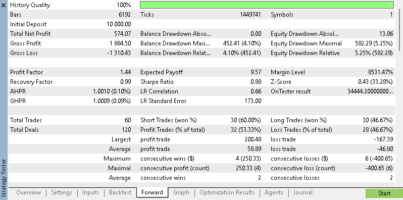
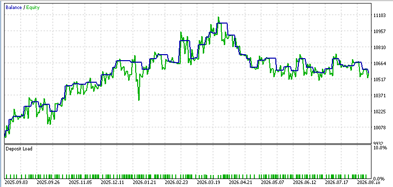
From our results above, it can be argued that further EURUSD 1-hour test-runs should try to map windows in the 96 to 160 region with a threshold in the 0.50 to 0.80 range. Being able to repeat these results over a slightly broad area in forward runs would matter more than a solo winning hit. A later revision could even add a normalized dominant amplitude or spectral concertation as a separate gate. Such an extra input could help separate a clear cycle from a weak phase.

The RSI, SNN, and MACD settings were dormant in this test run and should thus be excluded in follow up runs exploiting this route. Their inclusion would only create duplicate passes.

Mode-1

Our second operation mode moves the DFT onto the GBPJPY 2-hour timeframe while using the MACD main line. Optimization picked an 88-bar window which spans 176 price chart hours. The phase threshold was 0.35 which meant we accepted a wider part of the estimated cycle than Mode-0. The MACD filtered price through the slow and fast moving averages while the DFT window added a layer of memory.  The second mode is scored by our Trade Robot as follows:

//+------------------------------------------------------------------+
//| MODE 1: DISCRETE FOURIER TRANSFORM ON BASE MACD BUFFERS          |
//| Description: Extracts raw technical oscillator data vectors to   |
//|              isolate underlying cycle shifts in velocity.        |
//+------------------------------------------------------------------+
int ExecuteFourierMACD()
  {
   double macdValues[];
   ArrayResize(macdValues, InpFourierWindow);
   if(CopyBuffer(hMACD, MAIN_LINE, 0, InpFourierWindow, macdValues) < InpFourierWindow)
      return 0;
   double cycleState = CalculateFourierTurningPoint(macdValues);
   if(cycleState < -InpTurningPointTh)
      return 1;
   if(cycleState > InpTurningPointTh)
      return -1;
   return 0;
  }

This overlap is important. The retained MACD periods of 12 and 26 set how quickly momentum gets into the current analysis data vector, while the Fourier window size sets what proportion of this vector competes for the dominant frequency. A slow MACD and long window could delay the signal twice. Shortening both could turn ordinary momentum noise into a cycle.

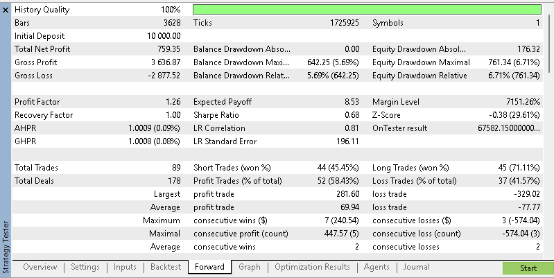
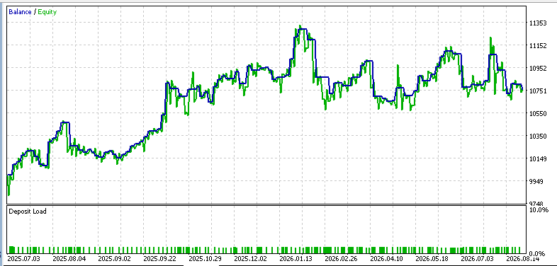
These positive test results are also reassuring given the positive forward walk. An alternative test run with XAUUSD on the 1-hour timeframe would give a harder transfer check because gold registers a whole new volatility, session and cost pattern. Four whole years typically feature several unique market phases. If we test the frozen inputs to begin with, we would then search a limited window range from roughly 64 to 112 bars prior to tweaking the MACD periods. Our target with running this on a paper account should also seek to bring some balance between longs and shorts because the original GBPJPY result was leaning heavily towards the former.

Mode-2

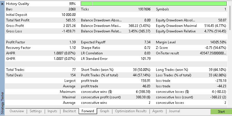
Our third mode changes RSI on the 4-hour timeframe as tested with AUDUSD. An RSI period of 14 feeds a 64-bar Fourier Window so that the route studies cycles in already smoothed momentum. This forward check was relatively clean, giving a Profit Factor of 1.39, a 4.77% maximum equity drawdown, a recovery factor of 1.10 while placing 77 trades. These figures make the case for further testing and proofing of this mode. This could stem from the argument that we do not know if the useful portion is the RSI, AUDUSD price action, or the sampled test window. Once again, to recap from the last related article, we use 'ExecuteFourierRSI()' in processing this mode as follows:

//+------------------------------------------------------------------+
//| MODE 2: DISCRETE FOURIER TRANSFORM ON BASE RSI BUFFERS           |
//| Description: Extracts raw momentum tracking arrays to decouple   |
//|              cyclical overextensions from market noise.          |
//+------------------------------------------------------------------+
int ExecuteFourierRSI()
  {
   double rsiValues[];
   ArrayResize(rsiValues, InpFourierWindow);
   if(CopyBuffer(hRSI, 0, 0, InpFourierWindow, rsiValues) < InpFourierWindow)
      return 0;
   double cycleState = CalculateFourierTurningPoint(rsiValues);
   if(cycleState < -InpTurningPointTh)
      return 1;
   if(cycleState > InpTurningPointTh)
      return -1;
   return 0;
  }

We had optimized to a 0.35 threshold that has a similar phase scale as what we had with the prior mode (Mode-1) given that the Fourier function returns a value rangebound to [-1,1]. The winning frequency could still be different since the RSI is bounded and usually lingers around its 50 mark. A paired grid of RSI periods from 8 to 28 and Fourier windows from 48 to 96 bars would indicate if the picked 14 and 64 are in a stable neighborhood.

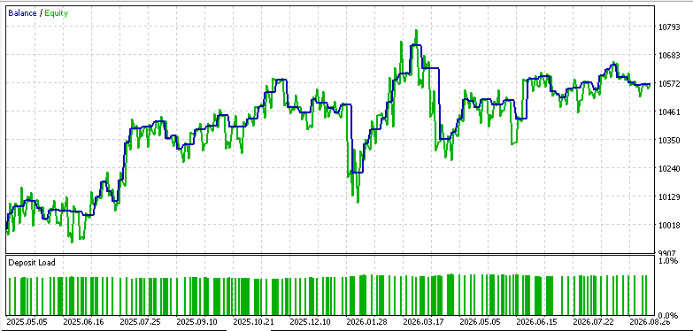
A follow up test of these results could be done with EURGBP on the 3-hour timeframe. Its relatively quiet price action would present the RSI with a different job that would avoid repeating the original 4-hour sampling interval. One trial could compare Fourier analysis of RSI levels to the analysis of the RSI first differences. The alternative checks cycles in the bar-to-bar change in RSI. MACD as well as SNN parameters would remain unchanged  since neither reaches its signal path.

Mode-3

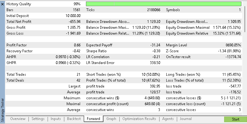
Our 4th mode brings together signals from price, MACD and RSI to test the USDCHF on the 6-hour timeframe. One 80-bar window and one 0.70 phase threshold rule all three branches prior to a two-out-of-three vote. Only 21 forward trades were made, we have a losing Profit Factor of 0.66 and an equity drawdown of 15.32%. Thus there is no case for paper account testing with this mode. Once again, as per the first article that introduced this algorithm-network pairing, we implemented this mode as follows:

//+------------------------------------------------------------------+
//| MODE 3: MULTI-LEVEL STRUCTURAL CYCLICAL CONFIRMATION             |
//| Description: Aggregates across price, momentum, and oscillator   |
//|              frequencies to locate total confluence turns.       |
//+------------------------------------------------------------------+
int ExecuteFourierCombined()
  {
   int consensus = ExecuteFourierPrice() + ExecuteFourierMACD() + ExecuteFourierRSI();
   if(consensus >= 2)
      return 1;
   if(consensus <= -2)
      return -1;
   return 0;
  }

The first thing to amend with this mode could probably be the sharing of inputs. Price, MACD and RSI do not need to have the same observation length or phase-gate. A revised Trade Robot would show or use a separate window-size and threshold for every data source. Testing every source separately and then freezing its acceptable range while still assessing price plus MACD, price plus RSI, and MACD plus RSI can then be performed. For this test run we did not use the SNN thus the threshold and input decay are dormant.

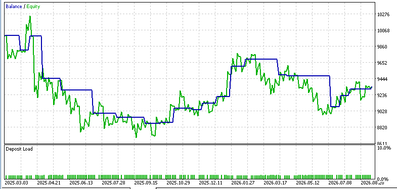
These amendments could be done by testing AUDJPY on the 4-hour timeframe. This slightly smaller timeframe increases our opportunity count while the Aussie cross gives us extended moves and reversals for the vote to work out. Any candidate giving less than 80 trades over five historical years should be rejected until the scores are checked. The paper-account testing phase should also log which component pair authorized each of the made entries. Without this, a nominal three-source model could prove to be just the same two voters appearing over and over again.

Mode-4

This mode is used to feed GBPUSD on the 30-minute timeframe candle measurements into the Spiking Neural Network. The optimized and proposed neural network inputs of 1.90 threshold and 0.60 decay leave 40% of membrane state for every price bar. These values were in one joint search. Candle bodies and the three-bar trend are raw price differences so an absolute threshold for issuing trades would not be stable over different price-action and volatility environments. Normalization of ATR, and the rolling volatility is needed to be done before more optimization is done. This mode was processed in MQL5, to recap, as follows:

//+------------------------------------------------------------------+
//| MODE 4: STRUCTURAL CANDLESTICK VELOCITY SPIKES                   |
//| Description: Extracts raw open/close metrics to detect sudden,   |
//|              explosive structural breakout momentum.             |
//+------------------------------------------------------------------+
int ExecutePriceActionSNN()
  {
   if(!InpUseSNN)
      return ExecuteFourierPrice();
   MqlRates rates[];
   if(CopyRates(_Symbol, _Period, 0, 3, rates) < 3)
      return 0;
   double bodyCurrent  = rates[2].close - rates[2].open;
   double bodyPrevious = rates[1].close - rates[1].open;
   double trendDelta   = rates[2].close - rates[0].open;
   return EvaluateSpikingNeuralNetwork(bodyCurrent, bodyPrevious, trendDelta);
  }

The forward walk report for this is also given below:

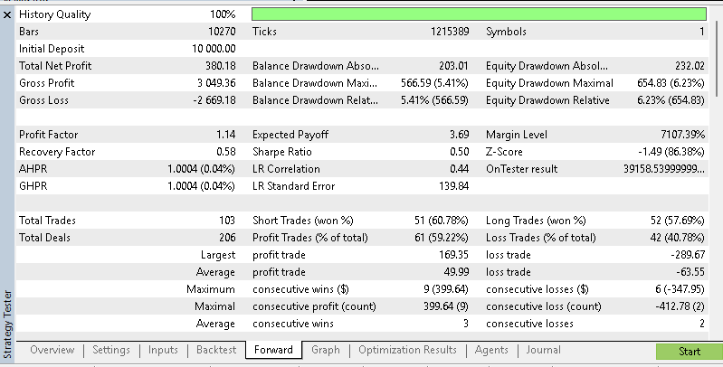
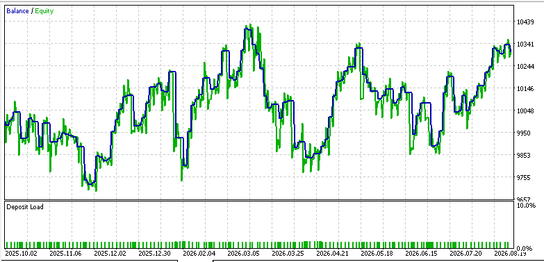
The forward walk report shows us over 100 trades with a Profit Factor of 1.14, and an equity drawdown 6.23%. As with many initial tests, this one has its doubts and a suitable paper account test could be with GBPJPY on the 15-minute timeframe. Larger intraday moves would give the candle room to separate different market regimes while the 15-minute timeframe could provide enough data points for analysis. We would record how often the neuron gives us signals. Sparse firing would require checks of input scale, decay and threshold. Frequent neuron firing should prompt a comparison with a basic threshold rule in order to help determine if accumulated states improve decisions. The suggested 0.5-5% range is an exploratory reference and ideally should be updated based on observed signal behavior. 

Mode-5

Our penultimate mode was used for testing the indicator-pattern SNN on USDCAD on the 8-hour timeframe. The optimized threshold of 0.30 with an equal decay of also 0.30 keeps 70% membrane state from one bar to the next. Our forward walk was in the red with Profit Factor just 0.74 and only 24 trades placed. We are testing the 7 modes in different situations to assess their robustness however it may be helpful to recap how we defined this mode in MQL5:

//+------------------------------------------------------------------+
//| MODE 5: TECHNICAL MOMENTUM SPATIAL DIVERGENCES                   |
//| Description: Maps differences between price structure layout and |
//|              RSI values to extract leading reversion signals.    |
//+------------------------------------------------------------------+
int ExecuteIndicatorPatternSNN()
  {
   if(!InpUseSNN)
      return ExecuteFourierCombined();
   double rsi[2], macd[2], closePrices[2];
   if(CopyBuffer(hRSI, 0, 0, 2, rsi) < 2)
      return 0;
   if(CopyBuffer(hMACD, MAIN_LINE, 0, 2, macd) < 2)
      return 0;
   if(CopyClose(_Symbol, _Period, 0, 2, closePrices) < 2)
      return 0;
   double rsiDelta  = rsi[0] - rsi[1];
   double macdDelta = macd[0] - macd[1];
   double priceDelta = closePrices[0] - closePrices[1];
   return EvaluateSpikingNeuralNetwork(rsiDelta, macdDelta, priceDelta);
  }

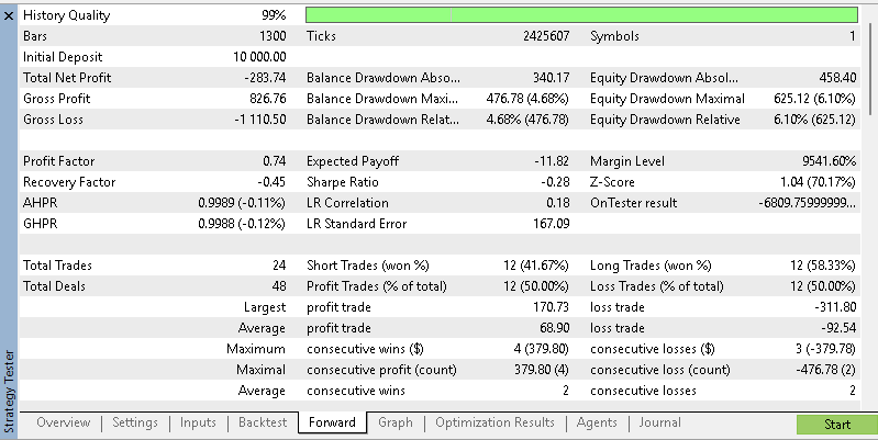
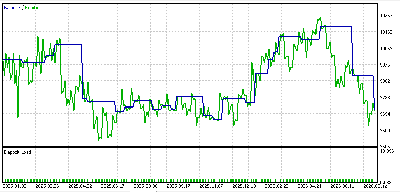
A Possible re-run of mode-5 could use NZDUSD at the 6-hour timeframe. This slower chart could leave enough time to get divergences while a different currency and session profile would test if the used membrane state can be relied on beyond USDCAD. In addition, this test run should have as many trades as possible, at least  25, in the optimized test window which could amount to half the paper-trading period. Once again in the demo-account/paper-trading runs, we would need to record every channel's signed contribution. No single signal source ought to dominate just because its units are larger.

Mode-6

The final mode of our exploration of various symbols, timeframes, and test windows; passes: 48-bar Fourier estimate, RSI momentum, and MACD momentum into the SNN on the EURUSD 15-minute timeframe. The analysis window spans 12 chart hours. With a threshold of 2.10 and decay of 0.10 we end up preserving 90% of the membrane state at each bar which lets small impulses to accumulate. This report gave us our best headline result with Profit Factor at 1.98, over 106 trades, and an equity drawdown of only 5.25%.

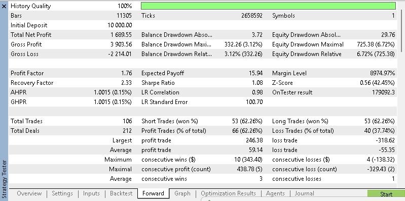
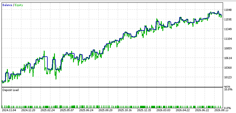
These results were attributed to how we implement in this mode in MQL5. A recap listing of this is given below:

//+------------------------------------------------------------------+
//| MODE 6: DUAL HYBRID ARCHITECTURE MATRIX                          |
//| Description: Couples long-wave Fourier cyclical models with      |
//|              leading momentum divergences to minimize false entries|
//+------------------------------------------------------------------+
int ExecuteHybridFull()
  {
   double closePrices[];
   ArrayResize(closePrices, InpFourierWindow);
   if(CopyClose(_Symbol, _Period, 0, InpFourierWindow, closePrices) < InpFourierWindow)
      return 0;
   double fourierPriceSignal = CalculateFourierTurningPoint(closePrices);
   double rsiValues[], macdValues[];
   ArrayResize(rsiValues, 5);
   ArrayResize(macdValues, 5);
   if(CopyBuffer(hRSI, 0, 0, 5, rsiValues) < 5)
      return 0;
   if(CopyBuffer(hMACD, MAIN_LINE, 0, 5, macdValues) < 5)
      return 0;
   double rsiMomentum  = rsiValues[0] - rsiValues[4];
   double macdMomentum = macdValues[0] - macdValues[4];
   if(InpUseSNN)
     {
      return EvaluateSpikingNeuralNetwork(fourierPriceSignal, rsiMomentum, macdMomentum);
     }
   else
     {
      if(fourierPriceSignal < -InpTurningPointTh && rsiMomentum > 0)
         return 1;
      if(fourierPriceSignal > InpTurningPointTh && rsiMomentum < 0)
         return -1;
     }
   return 0;
  }

The maximum balance drawdown was just 1.64% which was significantly less than the equity drawdown amount. Trades that were closed seemed smoother than the floating exposure between the exit and entry. That is a concern. In addition, scale was an issue. Given a balance drawdown of 1.64% versus an equity drawdown of 5.25%, it appears the trade account experienced deeper declines with open positions than the closed-trade record suggests. Further testing should help examine how long losing positions remain open and if a time-based exit could help reduce this exposure. 

The three inputs also get to the neuron on different numerical scales. The Fourier output range is [-1,1], RSI momentum uses oscillator points, and MACD momentum uses price units. RSI thus risks dominating the decision given that its [0,100] values are relatively large. Prior to refining the firing threshold of 2.10 or the decay of 0.10, a good test run would scale each input relative to its recent variability, this could then be followed by disabling one input at a time. This can help us know if Fourier, RSI, and MACD all contribute to the trading decision. 

An alternative symbol and timeframe for a further test run could be USDCAD at the 30-minute timeframe. Again the slower intraday chart changes the neural network accumulation and the loony brings a different session and spread formation as opposed to another broker-specific CFD. Testing out with random-delay or even a 25% spread hike could help prepare for worst-case scenarios. In this branch, enabling the SNN leaves InpTurningPointTh dormant because the Fourier phase passes directly into the neuron. MACDSignal is also inactive since we copy only the MACD main line. These two inputs should therefore be excluded from our optimization search, as changing them would have no effect on this route.

The OnTester function also needs a closer look across all modes. Multiplying trade count by net profit gives more weight to activity and nominal gain, while neither drawdown nor dependence on a narrow parameter region is directly penalized. Before ranking our candidates on a risk-adjusted basis, we should first apply minimum-trade and maximum-drawdown filters.

Results Summary

Our seven forward checks gave us five profitable settings and two losing ones. Mode-0 returned USD 574.07, Mode-1 returned USD 759.35, Mode-2 returned USD 565.55, Mode-4 returned USD 380.18, and Mode-6 returned USD 600.66. The losses were USD 655.94 for Mode-3 and USD 283.74 for Mode-5. Each figure belongs to its own test account and period, so we should keep these results separate. Adding them together would suggest a portfolio result even though we did not test the modes as a portfolio.

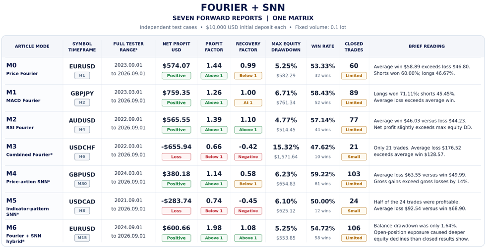
The first three Fourier-only routes all ended in profit, while the four SNN-active cases were evenly split between gains and losses. These results do not establish that the direct Fourier modes are better, given that each setting was different. What we can see is that neural gating did not make every feature set profitable. Allowing inputs to accumulate over several bars does not, by itself, resolve poor scaling or make an unhelpful input useful.

We also need to consider how many trades support each result. Our profitable 30-minute and 15-minute cases placed 103 and 106 trades, while the losing cases placed only 21 and 24. The smaller samples leave us with greater uncertainty. Even with that limitation, the USDCHF test on the 6-hour timeframe reached an equity drawdown of 15.32%, while the USDCAD test on the 8-hour timeframe held positions for more than eighteen days on average. Both settings still need revision.

The profitable runs also had weaknesses worth examining. GBPUSD on the 30-minute timeframe relied on its hit rate to offset larger average losses. EURUSD on the 15-minute timeframe showed a wide gap between balance and equity drawdown. Our GBPJPY 2-hour result leaned towards long trades, while EURUSD on the 1-hour timeframe leaned towards shorts. Looking only at the positive balance would leave these dependencies out of the assessment.

A further round of testing should change one element at a time. We could carry frozen parameters across adjacent forward windows to examine how the same settings behave over successive periods. Each SNN route could also be tested with its neural gate removed, keeping the symbol and dates unchanged. This comparison would help us determine whether the retained memory improved timing or simply changed how often trades were placed. Spread, commission and execution delay should then be increased without retuning the inputs.

These follow-up checks are beyond the scope of this article. Our reports give us five settings for another round of testing and two that require correction. Parameter stability, harsher trading costs and live evidence will still determine whether any of these candidates remains useful beyond the strategy tester.

Conclusion

In Part 6, we returned to the Fourier-SNN pairing after five introductory studies to explore how the same EA could behave across seven operating routes. Our tests moved from raw price cycles to transformed MACD and RSI, followed by the combined, price-action, indicator-pattern and full-hybrid SNN cases. Using different symbols, timeframes and test spans gave each mode a separate setting in which to examine its behavior.

The forward results were mixed, with five settings producing positive outcomes while USDCHF on the 6-hour timeframe and USDCAD on the 8-hour timeframe ended in losses. These losing runs are part of the assessment we need to make. They show where large adverse moves, weak payoff ratios and long holding periods were enough to overwhelm the selected trading logic.

Our model remains a research framework. Fourier analysis gives us a changing view of the dominant periodic structure, while the SNN retains state and delays action until the accumulated stimulation reaches a threshold. Neither component produces reliable information on its own. Their usefulness depends on the input series, sampling rate, calibration window and market phase in which we apply them.

Readers wishing to take this work further should repeat the forward process over rolling windows, keeping parameters frozen between periods. Testing each SNN route with the neural gate removed, together with harsher execution costs, would help establish what the model contributes. Some settings may improve through this process, while others may no longer hold up. We need this further testing before considering whether an EA built around the mechanism is suitable for live use.

The supplied source code and test results are intended for research and educational use. They are not investment advice and do not promise similar performance under live spreads, slippage, liquidity or future market conditions.

name	description
01 Fourier SNN RSI MACD.mq5	Custom Trade Robot coded to use FFT and Spiking Neural Network