Uncertainty as a Model (Part 2): Dependence Among Random Variables — From Correlation to Copulas

Table of Contents

1. Foreword
2. Introduction
3. Definition for the Multivariate Case
1. Multivariate Cumulative Distribution Function
2. Multivariate Probability Density Function
   
3. Analogy for Intuition
4. Simple Examples
5. Independence and Dependence
1. Definition
2. Marginal Distribution
3. Conditional Distribution
4. Independence as the Absence of Context
5. Conditional Expectation and the Regression Equation
6. Independence as the Meaninglessness of Prediction
7. Regression vs. Functional Relationship
6. Linear Theory
1. Covariance
2. Correlation
3. The Linearity Trap: What Does Covariance Leave Unsaid?
4. Linear Theory and the Multivariate Normal Distribution
5. Linear Theory in Action: Its Power and Its Limits
7. Copulas
8. Shannon's Theory
9. Conclusion
10. Appendix
11. List of Attached Files

Foreword

In the previous part, we discussed single random variables. However, a single variable is almost never sufficient to describe real-world market processes. In modern trading, virtually any task — from portfolio construction and hedging to identifying arbitrage strategies — boils down to assessing the joint behavior of many factors and assets. Therefore, a more sophisticated framework is needed — one that shifts the analysis from examining a single characteristic to modeling entire market structures.

This foundation also provides deeper insight into many other phenomena that are not directly related to trading. For example, large language models (LLMs) operate on the same principles. If their training is based on the maximum likelihood principle, then the mechanism of text generation is nothing more than the sequential computation of conditional probabilities in spaces of enormous dimensionality.

Introduction

A one-dimensional random variable is a function that maps outcomes ω from the space Ω to points x on the real line ℝ. Now we move on to a situation in which an entire family of variables coexists simultaneously in our probability space Ω: X1, X2, ..., Xn.

This transition can be compared to the evolution from analyzing individual points on a line to working with multidimensional vectors.

This is where the main pitfall for novice statisticians lies: in general, the distribution of a set of random variables cannot be described by a simple set of their individual distribution functions. Even if we know how asset A and asset B behave individually, we still know nothing about how they behave together. To fill this gap, we need the framework of multivariate distribution functions.

Key Definitions

Multivariate Cumulative Distribution Function

As before, the uppercase letter X denotes a random variable as a function defined on elementary events in a probability space Ω and taking numerical values in ℝ. The lowercase letter x denotes specific numerical values taken by X.

The multivariate cumulative distribution function for a set of variables X1, X2, ... , Xn is the probability that all the conditions Xi ≤ xᵢ are satisfied simultaneously:

F(x₁, x₂, ... , xₙ) = P(X1 ≤ x₁, X2 ≤ x₂, ... , Xn ≤ xₙ)

In the literature, you may encounter two terms that essentially describe the same thing: a multivariate cumulative distribution function and a joint cumulative distribution function. The difference between them is mainly stylistic and depends on the data structure. When we work with structures such as vectors or matrices (for example, the position of a particle in 3D space), we more often refer to a multivariate distribution of vectors or matrices. If, however, we analyze the relationship between several different variables (for example, inflation and the interest rate), the term “joint distribution” is more appropriate. From a mathematical standpoint, this is the same multivariate object, but this distinction is important for market modeling: it helps us understand whether we are viewing the system as a single entity or looking for hidden dependencies between different entities.

If in the one-dimensional case we intuitively visualized probability as a mass spread out along an infinite string (the axis X), then in the multivariate case our “unit mass” is distributed over a plane (for two variables) or throughout a volume (for three or more).

Multivariate distribution functions, like their one-dimensional counterparts, are rarely uniform. Mathematically, any distribution that is applicable in practice can be decomposed into two fundamental components: an absolutely continuous component and a singular component. There is an important terminological nuance here that often causes confusion:

• An absolutely continuous component is one in which probability is smoothly "spread" over the volume (area) of the space. For such distributions, a probability density function (PDF) always exists.
• The singular component is everything that is concentrated on sets with zero volume. This includes both the familiar discrete case (probability at points) and the more exotic continuous singularity.

Note. Going forward, for clarity, we will often limit our discussion to the two-dimensional case. The pile-up of subscripts is not entirely familiar to non-mathematicians, so instead of x's with subscripts in the two-dimensional case, we will use x and y for numerical values, and X and Y for random variables.

Visualizing a singularity in the plane: imagine a two-dimensional space (the XY plane).

• If the entire 100% probability mass is concentrated at individual points, then we are dealing with a discrete case (a zero-dimensional singularity).
• If the probability is distributed along a line (curve), this is a continuous singularity. The line itself has no area, but all the probability "lives" on it.

Why is this important for a trader? A singularity is always a sign of a rigid structure or constraint. If our data (for example, the prices of two assets) line up strictly along a single line, then there is a deterministic functional dependence between them (Y=f(X)).

Multivariate Distribution Density

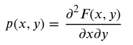
For absolutely continuous multivariate distributions, the concept of a joint probability density (Joint PDF) is introduced. If the distribution function (CDF) F(x, y) is the "cumulative total" of mass in a multidimensional region, then the density p(x, y) is the rate at which this mass accumulates at each specific point in space.

Mathematical definition: a multivariate density is obtained by successively taking the partial derivatives of the distribution function with respect to each variable. For the two-dimensional case (x and y), it looks like this:

An Intuitive Analogy

How should this be understood intuitively? If, in the one-dimensional case, density was a derivative (the rate of growth), then in the two-dimensional case it is a kind of “surface height” or the intensity of filling an area.
Imagine a terrain, and then:

• F(x, y) is the volume of soil in the rectangle extending from “negative infinity” to the point (x, y).
• p(x, y) is the elevation of the landscape at that specific point.

Where the density is high, we see “peaks” or “hills” of probability. For illustration, in trading, such hills on a “price–volume” or “price–volatility” chart clearly show clusters where the market is most stable or where trades occur most frequently.

An important point: just as in the one-dimensional case, the probability at a specific point (x, y) for a continuous distribution is always zero. Only the volume under the density surface over a specific region (for example, over a circle or a square in the plane) is meaningful. This volume will be the probability that a pair of random variables simultaneously takes values from this region.

Given a complete map of a multivariate distribution, we can easily derive distributions of lower dimensions from it — all the way down to individual one-dimensional series. In probability theory, this process is called finding marginal distributions.

Imagine our multivariate “probability cloud” in space. To see how a single variable (such as price) behaves while ignoring the others (volume, time), we simply “collapse” the cloud onto one of the axes. Mathematically, this is done by integrating (summing) the joint density over all “extra” variables.

However, here we encounter a critically important logical barrier: moving in the opposite direction is generally impossible.

The shadow principle: if we see the shadow of an object on a wall, we can roughly imagine its general contours, but we will never be able to unambiguously reconstruct the exact shape of this three-dimensional object.

Why is this important for data analysis? Knowing how often the price falls within range A and how often volume falls within range B is not enough to understand how they interact. There may be a rigid direct relationship, an inverse dependence, or a complete lack of correlation between them — at the level of “shadows” (one-dimensional distributions), all of this will look exactly the same.

This is precisely why, in data analysis, we move away from studying individual indicators toward examining their joint behavior.

Independence and Dependence

Definition

Building on the classical definition of independence of events (discussed in the article on elementary probability theory), we now turn to the independence of random variables. This is that rare and fortunate state of a system in which its components do not influence one another in any way.

Definition: two (or more) random variables are called independent if their joint cumulative distribution function factors into the product of their individual (marginal) cumulative distribution functions:

F(x, y) = Fx(x) * Fy(y)

If this equality is violated even in a small region of the plane, then the random variables are dependent by definition. For the continuous case, this rule carries over to densities. The joint density of independent random variables is simply the product of their densities:

p(x, y) = px(x) * py(y)

Marginal Distributions

Earlier, we discussed marginal distributions as “projections” of a multivariate cloud. Now let's see what this process looks like in mathematical terms. For simplicity, let’s consider the case of two random variables — X and Y — with their joint distribution function Fxy(x, y).

To obtain the individual (one-dimensional) distribution function for X, we need to “send Y off to the horizon.” Mathematically, this is equivalent to taking the limit as y → +∞:

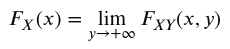
What's the logic behind this? When we ask, “What is the probability that X ≤ x for any value of Y?”, we are effectively removing the restriction along the second axis. The same works symmetrically for the random variable Y:

If, on the other hand, our joint distribution has a density pxy(x, y), then the transition to a one-dimensional world becomes even clearer. To find the density px(x), we must “sum” (integrate) the joint density over the entire Y-axis:

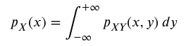
An intuitive model: imagine that the joint density is a three-dimensional landscape. To find the marginal density px(x), we imagine looking at this landscape from the side and “compressing” all the mountains and valleys into a single flat profile along a chosen axis.

Conditional distributions

The marginal distribution is often also referred to as the unconditional distribution. It describes the behavior of the quantity "in a vacuum," when we know nothing about other factors. But as soon as we fix the value of one variable (for example, learn the current trading volume y), the distribution of the second variable (the price x) changes instantly. This is what a conditional distribution is.

The easiest way to explain this concept is through probability density. If we have a joint density pxy(x, y), then the conditional density of the variable X, given that Y = y, is calculated using the formula:

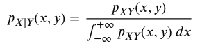
Please note: the denominator of this fraction is nothing other than the marginal (unconditional) density py(y), which we learned how to find in the previous step.

What does this mean intuitively? Imagine our "probability terrain" (the joint density). A conditional distribution is a vertical cross-section of this terrain along the line Y=y. We take a "knife" and cut through our landscape at the point where the value y is fixed. The resulting cross-sectional profile is the shape of the conditional density. Dividing by the integral (the denominator) is necessary only to “normalize” this slice — to ensure that the area under the resulting curve is once again equal to one.

In trading, this principle applies all the time: “What is the probability that the price will fall (X) if the volatility (Y) has already exceeded its average values?” The unconditional probability of a price drop may be 50%, but the conditional probability (given high volatility) may jump to 70%. These are precisely the shifts in probabilities that quantitative analysts look for when building their probabilistic models.

Independence as the Absence of Context

Now we can look at the concept of independence from a new perspective. If the random variables X and Y are independent, then knowing the value of one of them does not change our expectations about the other at all.
In this case, their conditional distributions coincide exactly with the unconditional (marginal) distributions:

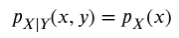
What does that mean in practice? Imagine that we are trying to predict a stock's return (X), based on the amount of rainfall in the Amazon (Y). If these variables are independent (which is logical for most tickers), then:

1. Our "unconditional" return estimate (marginal distribution) will provide a certain forecast.
2. Our "conditional" estimate (taking into account that there is heavy rain in Amazonia today) will yield exactly the same result.

Mathematically, this can be explained very simply: in the formula for conditional density, the joint density becomes the product of univariate densities pxy = px * py, and the “extra” density in the numerator and denominator of the conditional density formula simply cancels out.

Conclusion for the analyst: independence is a situation in which information about one factor has zero value for predicting the other. It is precisely the search for those conditions (Y) under which the conditional distribution (X) begins to noticeably “shift” relative to the unconditional distribution that constitutes the essence of the search for market patterns.

Conditional Expectation and the Regression Equation

Conditional distributions pave the way for calculating conditional means. These are exactly the same statistics we discussed for the one-dimensional case (expected value, variance, moments), but now they take into account the "context" of another variable.

The most important player here is the conditional expectation. It differs from the usual mathematical expectation only in that it ceases to be a constant and becomes a function of the value of another random variable:

My(x) = E[Y | X = x].

Mathematically, this is the dependence of the mean value of Y on the value taken by the random variable X. In science, this relationship has a generally accepted name: the regression equation. We should say a few words about standard notation. The notation E[A] is conventionally used to denote the expected value of a random variable A. The notation E[A|B] is used to denote the conditional expectation of A given B.

Intuitive meaning: if the ordinary expected value is the “average temperature in a hospital,” then the conditional expectation is the average temperature in a specific ward where patients with a certain diagnosis are staying.

Why is this very important?

• Forecasting theory: as a rule, a forecast is an attempt to calculate the conditional expectation of a future price (Y) given known current factors (X1, X2, ...).
• Machine learning (ML): if we look under the hood of modern neural networks or gradient boosting, we find that their main goal is to approximate this very conditional expectation as accurately as possible.
• Conditional volatility: conditional variance is calculated in a similar way — it is the basis for the GARCH family of models, which predict not the price itself, but risk (dispersion) depending on the current market state.

Thus, the simple formula for the conditional mean grows into a vast body of knowledge that enables the construction of predictive models of any complexity — from linear regression to large language models (LLMs).

Independence as the Futility of Prediction

In the world of independent random variables, the concept of prediction is reduced to something primitive. If X and Y are independent, then the conditional expectation becomes equal to the unconditional expectation:

E[Y|X=x] = E[Y]

This means that the regression equation becomes a boring constant — a horizontal line on the graph. What does this mean in practice? Here is another way to express the futility of independent data: if the variables are independent, then knowing the value of X does absolutely nothing to refine the prediction of Y.

• For a trader: if the return on an asset (Y) is independent of our indicator readings (X), then our “smart” conditional expectation (forecast) will always be equal to the historical average. Such an indicator does not narrow the range of uncertainty or shift the expected value in our favor.
• For data science, this is a zero-learning scenario. No matter how much data about X we feed into the model, it will not be able to produce a forecast any more accurate than the simple arithmetic mean of the target variable.

Thus, the entire industry of quantitative analysis is an endless search for situations where E[Y|X=x] ≠ E[X]. It is precisely in this difference that the potential profit lies.

Regression vs. Functional Relationship

It is important not to confuse the presence of dependence (when the regression equation differs from a constant) with a rigid (functional) relationship.

When we say that one quantity depends on another, we usually mean that knowing X helps us better predict Y. But in the vast majority of cases, Y still retains some of its random nature.

A rigid (functional) relationship is an extreme case where Y is uniquely and completely determined by X (for example, Y=2*X+5). From an intuitive standpoint (the geometry of masses that we discussed earlier), this is possible in only one scenario: a singular distribution. The entire probability mass on the XY plane “collapses” from a cloud into an infinitely thin line.

The “rigidity” criterion: in the case of a functional relationship, the conditional variance of one variable with respect to the other becomes zero. Var(Y|X=x)=0

What does this mean in practice?

1. In a general regression, we have a “cloud” of data points. The regression equation draws a line through the center of this cloud. However, there is still "noise" (conditional variance) around the line, and our forecast is probabilistic in nature.
2. In a functional relationship, the "cloud" no longer exists. There is only the line itself. Knowing X, we know Y with 100 percent certainty. The uncertainty disappears completely.

In trading, a true functional relationship is a rare occurrence. It occurs, if at all, in arbitrage (the relationship between futures and spot prices at expiration) or in synthetic instruments. In all other cases, we are dealing with a “soft” dependence, where the regression equation leaves the market room for a random maneuver.

Simple Examples

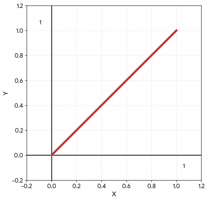
Below are three simple examples of bivariate distributions. Each example is accompanied by a diagram depicting its two-dimensional support (the set on which all probability is concentrated). In these cases, it is sufficient to show only the support in the figure, since the density is assumed to be “spread uniformly” over it.

Uniform on a square. The density is uniformly distributed over a square with sides parallel to the axes. The marginal distributions coincide with the conditional distributions and are one-dimensional uniform distributions on the interval [0,1]. The product of the densities of the marginal distributions is equal to the joint two-dimensional density itself, so the random variables X and Y are independent.

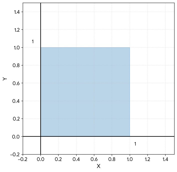
Uniform on a rotated square. Here, the conditional distributions of Y already depend significantly on x — they will be uniform distributions on different intervals. To understand this, it is enough to draw different vertical lines through the square — they will cut out different line segments within it. The marginal distributions will not be uniform at all. Therefore, the random variables X and Y are dependent. It is interesting to note, however, that the regression equations will turn out to be constants, just as they are when the variables are independent. In this example, the dependence between random variables is manifested in the dependence of the conditional variance of one variable on the value of the other.

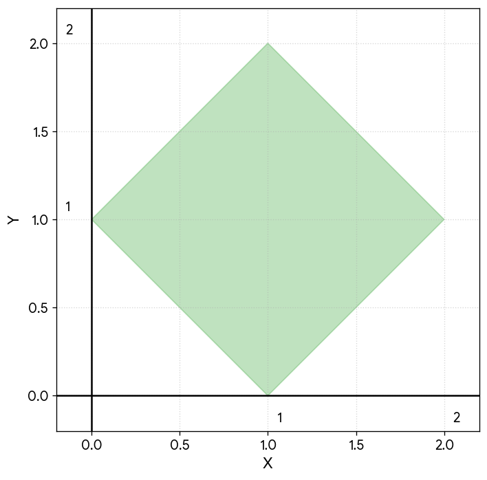
Singular on the line segment y = x. Here, there is an obvious functional relationship Y = X. The marginal distributions are uniform, while the conditional distributions are degenerate. The regression equation, of course, is identical to the functional relationship y = x.

The Appendix also includes examples of MQL5 scripts that generate three-dimensional density plots for a bivariate normal distribution and for several copulas (more on these below). The Appendix also includes MQL5 scripts for calculating parameters of marginal and conditional distributions and outputting two-dimensional plots of their densities.

Linear Theory

Covariance: a measure of joint movement

The first thing we define is a set (vector) of expected values m₁, m₂, ..., mₙ. It is simply a set of average values for each variable individually.

mᵢ=E[Xᵢ]

Next, we define the variances for each random variable:

varᵢ = E[(Xᵢ - mᵢ)²]

But now, in addition to the individual variances (measures of variation), for each pair of random variables Xi and Xj (where i ≠ j), we can calculate the covariance. It is defined as the average of the product of their deviations from their expected values:

What does that mean in practice? Covariance indicates the direction and magnitude of joint variability:

• Positive covariance: If both variables tend to deviate from their means in the same direction (they increase or decrease together), their product (xᵢ - mᵢ) * (xⱼ - mⱼ) will more often be positive.
• Negative covariance: If one variable increases while the other decreases, the product will be negative.
• Zero covariance: If the variables' movements are erratic relative to one another, their deviations will cancel each other out when averaged.

Intuitively: covariance is a "synchrony detector." For example, in trading, this is the basis of portfolio theory: if we buy two assets with high positive covariance, we do not diversify risk but rather double it, since they are likely to fall at the same time.

All possible covariances and variances of a set of variables are usually organized into a single square table — the covariance matrix. This is the "genetic code" of our data system: the variances are arranged along the diagonal, while the covariances (the relationships between the variables) are arranged off the diagonal.

Correlation coefficient: a universal scale

Covariance is an excellent tool, but it has a significant practical drawback: its value depends on the units of measurement. If we examine the relationship between the price of gold in dollars and volume in millions of contracts, the covariance will give us a huge number that says nothing by itself.

To correct for this, the (Pearson) correlation coefficient is used, which is essentially a normalized covariance. Mathematical definition: We take the covariance and divide it by the square root of the product of the variances (that is, by the product of the standard deviations).

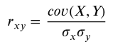
What makes it uniquely convenient? Thanks to this normalization, the correlation coefficient is always "confined" to a strict range from -1 to 1. This makes it the ideal ruler for measuring relationships:

• +1: A perfect direct relationship. The variables move in lockstep (a functional dependence).
• From 0 to +1: Positive relationship. The closer the value is to one, the more tightly the points cluster around a straight line. On average, an increase in one variable is accompanied by an increase in another.
  
• 0: There is no linear relationship. The variables "do not notice" each other (at first order).
• From -1 to 0: Negative relationship. The variables move in different directions: an increase in one indicates a tendency for the other to decrease.
• -1: Perfect inverse relationship / perfect negative correlation. One quantity is the mirror image of the other.

Intuitive meaning: the correlation coefficient does not tell us “how much” the variables increase together, but rather how closely they cluster around the regression line. The closer the value is to one (in absolute value), the less "noise" there is surrounding their joint movement, and the more reliable your linear forecast will be. As part of a preliminary ("at a glance") analysis in statistics, it is customary to use the following approximate correlation thresholds (absolute values are given):

• 0.1–0.3: Weak relationship.
• 0.5–0.7: A noticeable or strong relationship.
• 0.9+: Very high (nearly functional) dependence.

In trading, correlation is an important language for describing market structure. We construct correlation matrices to understand which assets move in tandem and which move in opposite directions.

The Linearity Trap: What Does Covariance Leave Unsaid?

The main reason covariance (correlation) has become the “gold standard” in statistics is its connection to independence. If two random variables X and Y are independent, then their covariance is guaranteed to be zero.

However, there is a tricky "but" that lies in wait for novice analysts here. The converse is generally false. Zero covariance does not necessarily imply independence. It simply tells us that there is no linear relationship between the variables.

• If the regression equation (the relationship between the variables) takes the form of a straight line, then the covariance will perfectly describe the strength of that relationship.
• But if the relationship is more complex (for example, quadratic or cyclical), the covariance may “go blind” and show zero, even though the variables are in fact rigidly linked to each other.

An intuitive example: imagine that the return on asset Y depends symmetrically on volatility X (when volatility is very low or very high, the return falls, and when it is in the middle, the return rises). On a graph in the XY plane, this will look like an arc. In this case, the covariance will show 0, cheerfully reporting a “lack of relationship,” even though a relationship is actually present — it is just nonlinear.

Linear Theory and the Multivariate Normal Distribution

We just said that zero covariance does not guarantee independence. However, there is one crucial exception upon which a good half of modern financial theory is based: the multivariate Gaussian (normal) distribution.

While a univariate normal distribution is defined by its expected value and variance, a multivariate normal distribution is determined by two analogous quantities:

1. The vector of expected values is the multivariate “center of gravity” of our cloud of points (the coordinates of the bell’s peak in space).
2. A covariance matrix is a generalization of variance. It not only shows the spread of each variable, but also determines the geometry of the cloud: how elongated it is and at what angle it is tilted.

In a “Gaussian world,” random variables behave in an extremely disciplined manner. The main feature of this distribution is that all the regression equations in it are always linear. There is no room here for intricate curves, arcs, or complex nonlinear relationships — only straight lines.

Let the random variables X and Y have a joint bivariate normal distribution with expected values mx and my, standard deviations sx and sy, and the (Pearson) correlation coefficient r. Then the conditional expectation E[Y|X=x] is expressed by the following regression equation:

E[Y|X=x] = my + r(x - mx)sy/sx

This leads to a fundamental consequence: if the joint distribution of a set of variables is a multivariate Gaussian distribution, then zero correlation is exactly equivalent to independence. Why is the linear approach the "holy grail" of modeling?

1. Mathematical transparency: for a normal distribution, the structure of the relationships is described completely and exhaustively by the covariance matrix. We do not need to look for hidden nonlinear effects — by definition, there simply are not any.
2. Simplifying the forecast: if the assets in our portfolio are Gaussian-distributed and their covariance is zero, we can be 100% certain that they do not influence each other in any way. A forecast for one asset will provide us with absolutely no information about another.

Linear Theory in Action: Its Power and Its Limits

The linear approach, based on covariances and correlations, has given rise to a whole universe of applied methods that are now considered the "gold standard" of analytics. Let's list some of them, formulating them in terms of random variables:

• Markowitz portfolio theory. A set of random variables (returns) with known means, variances, and covariances is given. A new variable (portfolio) is sought as a linear combination of the original variables. Moreover, this new variable must yield the smallest possible variance for every fixed value of its mean.
• Principal Component Analysis (PCA). For a given set of random variables, a new set is constructed from linear combinations of the original ones. At the same time, the new set must have a diagonal covariance matrix, and the elements on the diagonal must be sorted in descending order.
• Linear regression models: This is a fundamental modeling method in which the target variable (for example, the future price of an asset) is represented as a linear combination of explanatory factors (features, in machine learning terminology).

What's the catch in trading? Most of these models assume that the market is normally distributed. In this case, covariance becomes a complete measure of dependence. The problem is that real-world market data often exhibit "heavy tails" and nonlinear relationships that go beyond the Gaussian distribution. But it is essential to understand this “ideal case”: it is the reference point from which we measure any market anomalies. If the covariance is zero but a dependence is still detected, it means we have left the cozy Gaussian world and encountered the real complexity of the market.

Copulas: The Pure Architecture of Dependence

In the previous chapters, we saw that a joint distribution is a complex mix of the individual properties of variables and the relationships between them. Copulas (from the Latin *copula*, meaning “link” or “connection”) allow for a “surgical separation”: setting aside the characteristics of each individual variable and focusing exclusively on the structure of their relationship.

How does it work? By definition, a copula is a multivariate distribution in which all one-dimensional “shadows” (marginal distributions) are uniform on the interval [0; 1]. To bring any multivariate continuous distribution into this form, we use an elegant mathematical trick. We replace the values of each variable Xi with the values of its own distribution function: Yi=F(Xi). This is similar to feature normalization in machine learning. As a result, we obtain variables that “live” strictly from 0 to 1, while their individual differences (tails, skewness, and excess kurtosis) are canceled out.

The main strength of these models is their universality. Unlike linear methods, copulas allow you to work with any distributions and dependencies, even the most exotic ones. We can combine the “fat tails” of one asset with the “narrow peak” of another—the copula will describe their relationship without distortion.

The copula formula C(y1, y2, ...., yn) is directly determined by the type of dependence:

• Independence: If the variables are not related in any way, the copula turns into a simple product: C=y1*y2*...*yn.
• Complex relationships: For different dependence scenarios (for example, when assets are more tightly linked during a downturn than during an upturn), there are special families of copulas (Archimedean, Gaussian, Student’s t, etc.).

Intuitive model: A copula is a kind of “glue” that binds individual marginal distributions into a single whole. By studying the copula, an analyst sees the very geometry of this glue: where it bonds firmly (a rigid relationship) and where it allows the parts to move freely. If a covariance matrix is a simple ruler, then a copula is a full-fledged 3D scanner of relationships.

In modern market analysis, copulas are used, for example, in modeling systemic risk. They help us understand why, during market crashes, assets that seemed independent suddenly begin to behave as a single, unified whole.

When discussing copulas, it is impossible not to mention their role in the 2008 mortgage crisis. The term "The Formula That Killed Wall Street" has gone down in history — it refers to the widespread and inappropriate use of models based on the Gaussian copula. These models systematically underestimated the risks of simultaneous default by a large number of borrowers, which was one of the catalysts for the global collapse.

It is important to understand that the problem lay not in the mathematical theory itself, but in its blind application to processes that did not conform to it. For the discipline itself, this crisis served as a powerful catalyst for development. Today, this is a highly technical area of statistics that offers advanced tools such as "vine copulas" (Vine Copulas), which allow complex hierarchical dependencies in portfolios of hundreds of assets to be modeled flexibly.

The appendix to the article includes graphs (and the MQL5 scripts that generate them) of two two-dimensional copulas — the Gaussian copula and the Clayton copula — as examples.

Shannon's Theory: Entropy and Mutual Information

Traditionally, these concepts are found in textbooks on communications and data transmission. However, they are of interest to us as a universal measure of dependence between discrete random variables.

Shannon Entropy: A Measure of Chaos. Before measuring dependence, we need to measure the “amount of uncertainty” in the variable itself. To do this, we use Shannon entropy H(X). For a discrete random variable X, taking values with probabilities pi, entropy is calculated as:

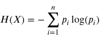
Now we can define mutual information I(X, Y). By definition:

I(X, Y) = H(X) + H(Y) - H(X, Y),

where H(X, Y) is the entropy of their joint distribution (the overall chaos of the system). The main properties of this indicator are:

• Zero under independence: if X and Y are independent, then I(X, Y) = 0. They do not share any information with each other.
• It is always positive in the case of dependence: if there is even the slightest relationship, the mutual information will be greater than zero.
• Universality: mutual information “sees” what correlation misses. If one variable is intricately intertwined with another, correlation may be zero, while mutual information will clearly indicate the presence of a relationship.

When defining entropy, it is permissible to choose a logarithm with an arbitrary base b > 1. When b=2 (binary logarithm), the values of entropy and mutual information are expressed in bits. In this metric, the entropy H(X) is interpreted as a measure of the prior uncertainty of a random variable or, equivalently, as the average amount of information obtained when a specific outcome occurs.

For a deterministic random variable (P = 1 for one of the states), the entropy is identically zero, since the outcome carries no new information. Maximum entropy is achieved for a uniform distribution, which characterizes the state of greatest uncertainty in the system. Within this information-theoretic framework, the mutual information I(X, Y) quantitatively describes the reduction in the uncertainty of one random variable given the realization (observation) of the value of the other.

In addition to absolute values, the analysis uses normalized mutual information U(Y|X) = I(X, Y)/H(Y), also known as the uncertainty coefficient (Uncertainty Coefficient). This dimensionless measure characterizes the proportion of uncertainty in the target variable Y that is eliminated when the value of the feature X is obtained, and it takes values in the range from 0 to 1. A value of U(Y|X) =0 indicates that the variables are statistically independent, whereas U(Y|X) =1 indicates complete determination of Y by the value of X.

In some ways, U(Y|X) is similar to the correlation coefficient, but it is always non-negative and can be used to identify nonlinear dependence. This coefficient is most effective when comparing the predictive power of features of different types, as it allows us to assess the relative contribution of each factor to reducing the entropy of the target variable.

The application of information measures to continuous random variables requires conceptual clarification, since the standard formula for discrete distributions does not apply in this case. The main approaches are:

1. Discretization (binning). A continuous range of values is divided into finite intervals (bins), which reduces the problem to the analysis of discrete quantities. This method is simple to implement, but its results depend critically on the choice of interval width: an interval that is too narrow leads to noisy estimates, while one that is too wide results in the loss of informative relationships.
2. Differential entropy. Integrals over the density function are used instead of sums. It is important to note that differential entropy is not a direct analogue of discrete entropy: it can take on negative values and is not invariant under coordinate transformations.

Unlike copulas, which large institutional players use for careful rebalancing of long-term portfolios, information theory tools have found their place at the forefront of HFT (High-Frequency Trading). In a world where lightning-fast algorithms engage in fleeting battles, classical correlation is too slow and blind. Here, mutual information is used to instantly detect nonlinear microstructural dependencies that exist for only fractions of a second.

The modern arsenal of high-frequency trading includes such advanced concepts as transfer entropy (Transfer Entropy), which allows us to assess not just the presence of a relationship, but the directional flow of information from one asset to another (which one is the “leader,” and which is the “follower”). To calculate these quantities in practice using noisy market data, effective nonparametric approaches are used, such as the KSG algorithm (KSG estimator, named after its authors Kraskov, Stögbauer, and Grassberger). These methods allow algorithms to “sense” the market's pulse and make decisions in situations where more traditional statistical models have not yet detected a change in the situation.

The Appendix to this article contains an MQL5 script that calculates and displays all entropies (H(X), H(Y), H(X, Y)) and their mutual information (absolute I(X, Y) and relative U(Y|X)) for the joint distribution of two discrete variables, each taking two values.

Conclusion

We have examined how random variables form unified structures in multidimensional space, and how their relationships take on geometric form. But in trading, we never know their true parameters in advance — we only have historical price data, which is a limited sample. How can we use this sample to reconstruct the actual picture, and to what extent can we trust the figures obtained? The fundamental laws of probability theory — the Law of Large Numbers and the Central Limit Theorem — help us find the answer. In the next part, we will move from probability theory to mathematical statistics, where we will estimate parameters and test hypotheses, continuing to draw on the capabilities of the MetaTrader 5 platform and the MQL5 language.

Appendix: Practical Implementation in Code

Appendix 1

The gauss_3D.mq5 script visualizes a 3D plot of the bivariate probability density function (PDF) for a normal distribution with specified parameters. The graph also shows the regression line of Y on X. The regression equation is also shown in analytical form. Blue represents the density, red represents the coordinate axes, and green represents the regression line of Y on X.

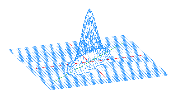
For a bivariate normal distribution with parameters:
Expected value of X: 0.000
Expected value of Y: 0.000
Standard deviation of X: 1.500
Standard deviation of Y: 1.500
Correlation coefficient between X and Y: 0.800
Regression equation: E[Y|X=x] = 0.000 + 0.800 * x

Appendix 2

The marginal.mq5 script calculates parameters and plots the probability density functions (PDFs) of the marginal distributions for a bivariate normal distribution with specified parameters. These distributions are also normal, but univariate.

It is interesting to note that the parameters of the marginal distributions X and Y do not depend on the correlation coefficient between these random variables. This is yet another confirmation that univariate distributions of random variables do not reflect the relationship between them.

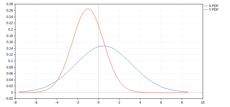
For a bivariate normal distribution with parameters:
Expected value of X: 0.500
Expected value of Y: -1.000
Standard deviation of X: 2.700
Standard deviation of Y: 1.500
Correlation coefficient between X and Y: 0.800
The marginal distribution of X has the following parameters:
Expected value: 0.500
Standard deviation: 2.700
The marginal distribution of Y has the following parameters:
Expected value: -1.000
Standard deviation: 1.500

Appendix 3

The conditional.mq5 script calculates parameters and plots the density functions (PDFs) of the conditional distributions Y|X=x₁ and Y|X=x₂ for given x₁ and x₂ for a bivariate normal distribution with specified parameters. These distributions are also normal, but univariate.

Unlike marginal distributions, conditional distributions depend on the correlation coefficient: the higher the correlation coefficient, the lower the conditional variance. In the limiting case where the correlation coefficient equals one, the conditional variance goes to zero and the conditional distribution becomes degenerate: the dependence of Y on X becomes a deterministic functional dependence.

For a fixed (nonzero) correlation coefficient, the conditional distribution of Y depends on the value of X, but this dependence affects only the expected value. The variance remains the same. In statistics, this property of constant conditional variance is commonly referred to as homoscedasticity (while non-constancy is referred to as heteroscedasticity). Linear regression models are well suited (especially when the classical least-squares method is used to estimate their coefficients) for modeling under homoscedasticity, but real-world data are almost always heteroscedastic.

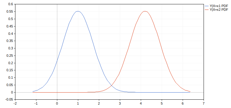
For a bivariate normal distribution with parameters:
Expected value of X: 0.000
Expected value of Y: 1.000
Standard deviation of X: 1.000
Standard deviation of Y: 2.000
Correlation coefficient between X and Y: 0.800
The conditional distribution of Y given X = 0.000 has the following parameters:
Expected value: 1.000
Standard deviation: 0.720
The conditional distribution of Y given X = 2.000 has the following parameters:
Expected value: 4.200
Standard deviation: 0.720

Appendix 4

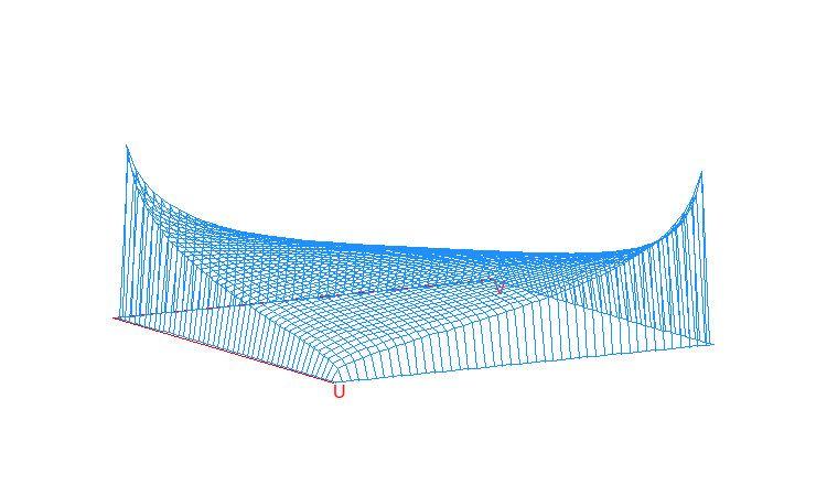
The copula_gauss.mq5 script visualizes the probability density of a Gaussian copula. The use of the symbols U and V instead of the traditional X and Y is due to the specifics of copula theory: the symbols x and y denote the original variables, whereas u and v denote their values transformed through the corresponding marginal distribution functions (CDFs).

The viewing angle of the 3D projection is chosen so that the leftmost point of the graph corresponds to the origin (0, 0), which represents the left tails of the distributions (negative infinity for the original variables). The opposite point corresponds to the region (1, 1), that is, the right tails (positive infinity). The height of the graph is directly proportional to the strength of the relationship in that region. The Gaussian copula is characterized by symmetric peaks in both corners, indicating the same dependence structure both when assets fall together and when they rise together.

Appendix 5

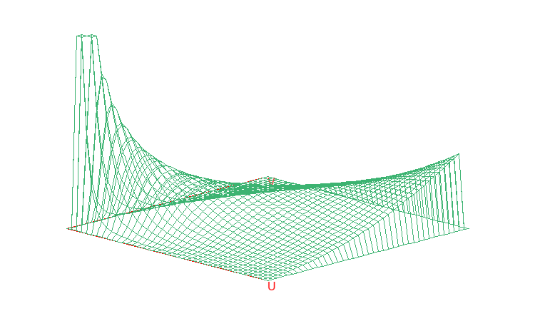
The copula_clayton.mq5 script visualizes the probability density of the Clayton copula (in the same projection as in the previous appendix). A key feature of this distribution is its pronounced asymmetry: in the region of the origin (0, 0) there is a significant density peak, whereas at the point (1, 1) no such spike is present.

This geometry of the graph indicates strong lower-tail dependence, in which the probability of a simultaneous extreme decline in assets is significantly higher than the probability of their simultaneous rise. Such an asymmetric structure cannot be described using the standard linear Pearson correlation coefficient, which makes the Clayton copula an indispensable tool for modeling systemic risk and market crashes.

Appendix 6

The shannon.mq5 script calculates and outputs all entropies (H(X), H(Y), H(X, Y)) and mutual information (absolute I(X, Y) and relative U(Y|X)) for two discrete variables X and Y, each taking two values (x1 and x2 for X; y1 and y2 for Y). The specific numerical values of the random variables are not important for the calculations, so letter symbols are sufficient.

Specified joint distribution probabilities:
for (x1, y1): 0.30, for (x1, y2): 0.10, for (x2, y1): 0.20, for (x2, y2): 0.40
Calculated statistics:
Entropy of X, H(X): 0.97
Entropy of Y, H(Y): 1.00
Joint entropy of X and Y, H(X, Y): 1.85
Mutual information between X and Y, I(X, Y): 0.12
Uncertainty coefficient, U(Y|X): 0.12

Attached files

#	name	Description
1	gauss_3D.mq5	The script plots a 3D graph of the bivariate density (PDF) for a normal distribution with specified parameters. It also displays the regression line and shows the form of the regression equation.
2	marginal.mq5	The script calculates parameters and plots the probability density functions (PDFs) of marginal distributions for a bivariate normal distribution.
3	conditional.mq5	The script calculates parameters and plots the density functions (PDFs) of conditional distributions for the bivariate normal distribution.
4	copula_gauss.mq5	The script visualizes the probability density function of a Gaussian copula.
5	copula_clayton.mq5	The script visualizes the probability density function of the Clayton copula.
6	shannon.mq5	The script calculates and displays the entropy and mutual information for the joint distribution of two discrete variables, each taking two values.