

Recovering Option-Implied Probability Distributions Across Four Markets in MQL5
 112
112
 0
0

Introduction
A single number can hide a great deal. Ask the options market how much an instrument might move over the next month, and it answers with one figure, an implied volatility. That figure is informative, and it is also a compression. One number describes a whole set of possible outcomes, and it describes them faithfully only if those outcomes are shaped the way the pricing model assumes.
They are not, and the chain says so. Options struck far below the money trade at higher implied volatilities than options struck at the money, which is another way of saying the market does not believe in the tidy lognormal outcome that one number stands for. On the GLD reading below, the recovered distribution has a kurtosis of 7.4, against 3.1 for a lognormal distribution with the same at-the-money volatility and 3.0 for a normal one.
So, the chain contains more than a single volatility. It also implies a full terminal probability distribution, recoverable from the quoted prices by an identity nearly fifty years old. The output is a set of price levels with a probability attached to each one. I pulled one number out of a chain like this in an earlier article and set it against what the market had actually been doing. Writing it left me with a question I could not drop. That one number assumes a shape for the outcomes, and I wanted to know which shape the chain was actually pricing. I went back to the same data and took the whole distribution instead. It turned out useful enough to keep on my chart, and that is what this is.
The chain that gets read here is GLD, the gold ETF, so what comes out is a distribution of GLD. But the method is not about gold, and the article does not ask you to take that on faith: the same unchanged pipeline is run on SLV, SPY, and USO, on two separate afternoons, and every reading is published with its diagnostics. Their connections to XAUUSD, XAGUSD, US500, and USOIL are proxy mappings for monitoring, not equivalences.
By the end you will have three programs and the class library the service is built on. (1) A Python script that reads an ETF option chain, recovers the implied distribution, and writes its percentiles to a small file. (2) An example MetaTrader script that reads the file and prints those percentiles as prices on your own symbol. (3) A background service that draws the levels on a chart and sends a phone notification when price leaves the risk-neutral 5 to 95 percent band implied by the options. The service keeps its logic in a class library, ImpliedDensityMonitor.mqh, which is the fourth source file. All of it is source code you can read and change. It never trades.
From option prices to probabilities
Start with a column of call prices. A higher strike gives a smaller payoff region, so calls become cheaper as the strike rises. Where that price curve bends sharply, more probability sits between neighboring strikes; where it barely bends, less does.
Breeden and Litzenberger made that statement exact. Differentiate the call price with respect to strike once and you obtain the discounted tail probability. Differentiate again and undo the discounting to obtain the terminal density. The curvature of the call price curve is therefore the implied probability density, strike by strike. [1]
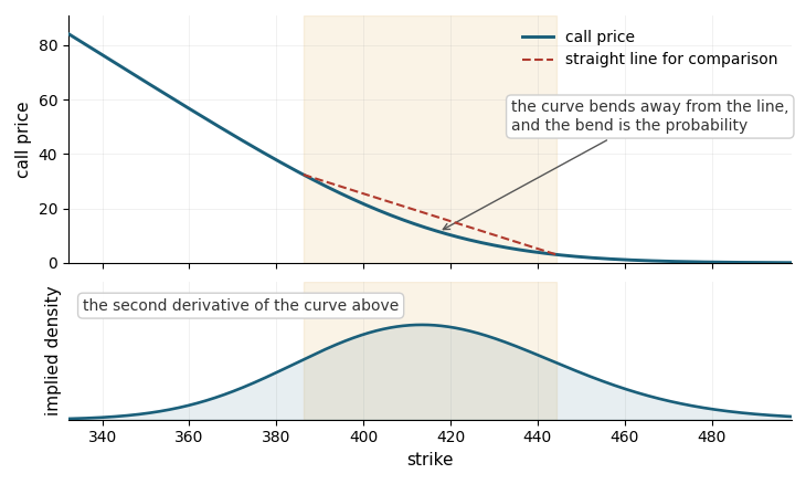
Call prices fall as the strike rises, and the curvature of that fall is the implied probability density. This illustration uses a single volatility so the mechanism is visible on its own; real quotes can produce a different and less stable tail shape.
A volatility surface reports how each option is priced; the density reports what those prices jointly imply about the underlying. Recovering it requires the chain rather than one volatility, and differentiation amplifies every stale print and wide spread. Raw quotes must therefore be filtered and smoothed before the second derivative is taken. [4] [5]
Two restrictions on everything that follows
The first restriction is the measure. Option prices produce a risk-neutral density, not a real-world forecast. Investors pay for protection, and that premium is embedded in the recovered tails. [3]
So, a 5th percentile means the market is priced as though five percent of the probability sits below it. It does not state a five percent real-world probability. Converting between the two measures requires assumptions about risk preferences and is outside this build.
The second restriction is the underlying. GLD, SLV, SPY, and USO are exchange-traded instruments, while a broker may quote XAUUSD, XAGUSD, US500, and USOIL. Their hours, structures, fees, and financing differ. USO is the weakest mapping because it holds and rolls oil futures; GLD and SLV remain ETF proxies for spot metals; SPY is not the broker's index CFD. Rescaling provides context but never makes the distributions native to those local symbols.
Recovering the density in practice
The identity assumes an arbitrage-consistent call curve, while market quotes are discrete and noisy. The first task is therefore to turn the chain into a smooth curve without hiding what was repaired.
The forward comes from put-call parity rather than from spot compounded at the risk-free rate. That avoids assuming away dividends, fund fees, storage economics, or futures roll effects. Each strike quoted on both sides gives a forward estimate; the script takes the median of the eight strikes where calls and puts are closest in price and publishes their spread. In the GLD feed collected at 2026-09-14T13:53:39Z, the forward was 393.2060 against spot at 392.25, with a parity spread of 0.0410 percent.
Black-76 then places out-of-the-money puts below the forward and calls above it in one pricing space. [7] The script solves their implied volatilities and fits a smooth curve in forward log-moneyness. It then reprices a dense synthetic call grid, takes the second difference, undoes discounting, normalizes the density, and converts it to percentiles.
Three of those steps involve choices rather than measurements, and pretending otherwise is where this kind of work usually goes wrong.
The first is the smoothing. Fitting in volatility rather than in price is what makes it safe, because prices across strikes span orders of magnitude while implied volatilities live in a narrow band. But a smooth smile does not guarantee an arbitrage-consistent call curve. It can produce a curve that is not convex, and a call curve that is not convex produces negative probability. So the degree is not fixed in advance. Every degree from three down is recovered in full, the negative mass each one leaves is measured, and the first specification that leaves less than 1 percent is used. That gate limits negative probability. It does not guarantee a convex call curve, and any convexity violations that remain are counted and published with the reading.
The second is how the fit weights its points. Two weights are multiplied. One concentrates the fit near the money, which is standard, and which quietly flattens the wings if it is too narrow. The other trusts a tight quote more than a wide one, because a bid-ask spread is evidence about how real a printed price is. The width of the first is a judgment, so it is not asserted; it is swept in the sensitivity study further on.
The third is what happens outside the quoted strikes, and it turned out to matter more than the degree. Holding volatility flat past the last quoted strike is the obvious choice, and it is what an earlier version of this did. It is also crude: where a sloped polynomial meets a flat extension there is a kink, a kink in the volatility curve becomes a non-convex spot in the call curve, and that shows up as negative probability. Instead, extending total variance linearly using the edge slope produces a smooth join. On live quotes the difference was stark. Across the fifty-four specifications recovered on the GLD reading below, the worst specification left 4.74 percent of negative mass. The smooth rule at degree three, which is what the feed publishes, left 0.004 percent. Negative mass is measured throughout as a share of the gross absolute mass, the positive and negative parts added together. For small values that is practically the same as a share of total probability; the 4.74 percent worst case is about 5.2 percent of it.
That is the whole trap in miniature, and it cost me a version. My first density had a kurtosis of 11.6, because a polynomial evaluated far outside its data does not flatten out, it diverges, and it invents probability where no contract has ever traded. Naming a tail rule fixed that. Choosing the tail rule that does not kink fixed what the naming left behind.
Thresholds are judgment, not physics. Contracts are kept when they have an open interest of at least ten, a live two-sided quote that is not crossed, a price above five cents, a bid-ask spread under a quarter of the mid, and a strike between 80 and 120 percent of the forward. The section on how far to trust each number measures what those thresholds cost.
Implementation of the density feed in Python
MetaTrader cannot read these option chains, so the recovery happens outside and the terminal is handed the answer. The script accepts an ETF through "--ticker", extracts its forward, solves implied volatility for every surviving contract, fits the smile, recovers the density, checks it for arbitrage, and writes one small JSON object. Each instrument gets its own flat file, such as feed_gld.json or feed_spy.json, so the hand-written MQL5 parser remains unchanged. The output is relative rather than absolute: the feed publishes each percentile as a multiple of the forward, together with the forward and the spot.
The terminal multiplies each ratio by forward over spot, which turns it into a multiple of the ETF spot, and only then applies it to the spot-like local price. That keeps the ETF's own carry out of the mapping. The local symbol's carry, sessions, and funding still differ, which is one reason the mapping stays a proxy.
# the command-line default. Every downstream calculation uses this selected ticker
DEFAULT_TICKER = "GLD"
TICKER = DEFAULT_TICKER

# labels travel with the feed so the ETF-to-terminal mapping is never hidden
UNDERLYING_NOTES = {
    "GLD": "GLD ETF proxy for gold, not spot gold or broker XAUUSD",
    "SLV": "SLV ETF proxy for silver, not spot silver or broker XAGUSD",
    "SPY": "SPY ETF proxy for the S&P 500, not a cash index or broker US500 CFD",
    "USO": "USO holds oil futures; it is not spot crude or broker USOIL",
}

# four percent is a transparent discount-rate input, not a carry assumption; the
# forward and net carry are recovered independently from put-call parity
RISK_FREE = 0.04

# liquidity filters: 10 contracts and a five-cent price reject empty penny wings,
# while a 25 percent relative spread keeps only quotes with a meaningful midpoint
MIN_OI = 10
MIN_PRICE = 0.05
MAX_SPREAD = 0.25          # reject a quote whose bid-ask spread exceeds this of its mid

# 80 to 120 percent of the forward keeps the liquid core and enough wing curvature
# without letting remote penny strikes dictate the fit
MONEY_LO, MONEY_HI = 0.80, 1.20

# two to 200 percent accepts plausible ETF regimes while rejecting solver-boundary
# values that indicate an inconsistent price rather than a measured volatility
IV_FLOOR, IV_CEIL = 0.02, 2.00

# 20 to 45 days brackets the article's one-month target without selecting a very
# short gamma-dominated expiry or jumping to the following quarter
EXPIRY_LO, EXPIRY_HI = 20, 45

# the 55 to 165 percent grid reaches beyond the fitted strikes, while 2,200 steps
# keep the flat-smile percentile error below three basis points in the self test
GRID_LO, GRID_HI = 0.55, 1.65
GRID_STEPS = 2200

# degree three permits ordinary skew and curvature without high-order oscillation;
# width 0.35 keeps the center influential, and eight points across four percent of
# the forward is the minimum span allowed to support a curve rather than a line
FIT_DEGREE = 3
FIT_WIDTH = 0.35
MIN_POINTS = 8
MIN_SPAN = 0.04

# outside the quoted strikes the fit must not be extrapolated. The live feed does not
# read this default: choose_fit tries linear total variance first, falls back to flat,
# and publishes the rule it used. The default only applies when a caller names no rule
TAIL_RULE = "linvar"

# a recovered call curve that is not convex is not arbitrage-consistent, and the
# density it produces contains negative probability. The specification is chosen to
# leave the least negative mass, and the first one under this gate is taken. The gate
# does not guarantee convexity: remaining violations are counted and published
NEG_MASS_MAX = 1.0

# 30 completed sessions roughly matches the target option horizon; realized
# volatility is reported only as context, never substituted for the implied density
RV_WINDOW = 30

# the spot comes from a different request than the chain, so it can be stale while
# the options are current. Beyond this much implied carry it is stale, not financed
CARRY_MAX = 25.0

# the sensitivity study: every combination is recovered and the spread is published.
# FIT_WIDTH is included because a fit weighted hard toward the money can flatten the
# wings, which is exactly the region the recovery exists to measure
SENS_DEGREES = (2, 3, 4)
SENS_WINDOWS = ((0.75, 1.25), (0.80, 1.20), (0.85, 1.15))
SENS_TAILS = ("flat", "linvar")
SENS_WIDTHS = (0.20, 0.35, 1.00)

# the filter study: the liquidity thresholds are judgment, so their effect is measured
SENS_MIN_OI = (0, 10, 50)
SENS_MAX_SPREAD = (0.10, 0.25, 0.50)
Most constants are either liquidity filters or values swept later. The rate is used only for discounting; carry is measured from parity.
def forward_from_parity(chain, t_years, rate, debug=False):
    """
    Read the forward out of the market instead of assuming a carry.

    European put-call parity says C - P = exp(-rT) * (F - K) at every strike, so each strike
    quoted on both sides gives an estimate of F. The median over the strikes nearest
    the money is taken, which is robust to one bad quote.

    Nothing in here uses a spot quote. The strike nearest the money is the one where
    the call and the put are closest in price, which is a property of the chain
    itself. A spot that arrives late or stale therefore cannot move the forward, nor
    move which strikes are treated as being at the money, which is the mistake this
    replaced: the spot comes from a different request than the options do.

    This matters because an ETF need not be a non-dividend-paying asset in the pricing
    sense. Dividends, fees, storage, or futures-roll economics can make F = S * exp(rT)
    wrong and bias every volatility solved against it.

    Assumes that European put-call parity is an adequate approximation for these quotes.
    """
    cmap, pmap = strike_map(chain.calls), strike_map(chain.puts)
    common = sorted(set(cmap) & set(pmap), key=lambda k: abs(cmap[k] - pmap[k]))
    if len(common) < 3:
        raise ChainUnusable("fewer than three strikes quoted on both sides")

    disc = math.exp(-rate * t_years)
    estimates = [k + (cmap[k] - pmap[k]) / disc for k in common[:8]]
    fwd = float(np.median(estimates))
    if not math.isfinite(fwd) or fwd <= 0.0:
        raise ChainUnusable("put-call parity produced no usable forward")

    spread = (max(estimates) - min(estimates)) / fwd
    if debug:
        print("  forward %.4f from put-call parity over %d strikes, spread %.4f%%"
              % (fwd, len(estimates), 100.0 * spread))
    return fwd, spread
In its European form, put-call parity holds at every strike quoted on both sides, so each of those strikes gives its own estimate of the forward, and the median of the ones nearest the money is the estimate taken. For American ETF options it holds only approximately, which is one more reason for taking the median rather than any single strike. The spread across them is published too, because when they disagree the chain is telling you something about its own quality that no single number would.
The inversion is bisection rather than Newton-Raphson: an option price rises steadily as the assumed volatility rises, so a bracketed search cannot get lost, and a hundred halvings of a range from 2 to 200 percent narrow it far beyond the precision the result needs.
One small thing in that step fixes a bug that produced no error at all. The natural way to read a possibly missing quote is float(row.get("bid") or 0.0), and it is wrong. When a quote is missing, pandas returns NaN, and NaN is truthy in Python, so the fallback never fires and NaN flows into the solver instead of zero. Nothing raises. The contract simply disappears from the fit, quietly, and the density is built from fewer points than you think. One isfinite check ends it.
Then the smoothing, which is the step that decides whether the density is a measurement or an artifact.
def fit_smile(points, fwd, degree=FIT_DEGREE, debug=False, width=FIT_WIDTH):
    """
    Fit a smooth volatility curve in forward log-moneyness, and remember its range.

    Differentiating raw quotes twice turns bid and ask noise into a meaningless
    density, so the quotes are smoothed first. A low-degree polynomial keeps the
    dependencies to numpy and cannot oscillate the way a high-order spline can. It
    does NOT guarantee an arbitrage-free call surface, which is why the recovered
    curve is checked afterwards rather than assumed.

    Assumes points contain positive strikes, solved volatilities and relative spreads.
    """
    if len(points) < MIN_POINTS:
        raise ChainUnusable("only %d usable contracts" % len(points))

    strikes = np.array([p[0] for p in points], dtype=float)
    vols = np.array([p[1] for p in points], dtype=float)
    spreads = np.array([p[2] if len(p) > 2 else 0.0 for p in points], dtype=float)
    x = np.log(strikes / fwd)

    span = float(x.max() - x.min())
    if span < MIN_SPAN:
        raise ChainUnusable("the usable strikes span only %.3f in log-moneyness" % span)

    #--- two weights multiplied. The first concentrates the fit near the money, and a
    #--- narrow choice there flattens the wings, so its width is swept in the
    #--- sensitivity study rather than treated as settled. The second trusts a tight
    #--- quote more than a wide one, which is what a bid-ask spread is evidence about
    weights = np.exp(-(x / width) ** 2) / (1.0 + spreads / 0.05)
    for deg in (degree, degree - 1, 1):
        if deg < 1 or len(points) < deg + 3:
            continue
        try:
            coeffs = np.polyfit(x, vols, deg, w=weights)
        except (np.linalg.LinAlgError, ValueError):
            continue
        if not np.all(np.isfinite(coeffs)):
            continue
        if debug:
            print("  smile fitted at degree %d over %d points, span %.3f"
                  % (deg, len(points), span))
        return {"coeffs": coeffs, "xlo": float(x.min()), "xhi": float(x.max()),
                "degree": deg}

    flat = float(np.average(vols, weights=weights))
    if debug:
        print("  smile fit failed, falling back to a flat %.4f" % flat)
    return {"coeffs": np.array([flat]), "xlo": float(x.min()), "xhi": float(x.max()),
            "degree": 0}


def smooth_vol(fit, fwd, strike, t_years, tail=TAIL_RULE):
    """
    Evaluate the fitted smile at one strike, under an explicit tail rule.

    Inside the quoted range the polynomial is used. Outside it the fit must never be
    extrapolated, because a polynomial diverges past its data and invents probability
    mass. Two conventions are offered:
      flat    hold the edge volatility, which makes the far tails lognormal
      linvar  extend total variance linearly at the slope of the edge
    Neither is the market's opinion. The tails outside the quoted strikes are a
    convention, and the sensitivity study measures how much that convention matters.

    Assumes fit contains polynomial coefficients and finite fitted-range endpoints.
    """
    x = math.log(strike / fwd)
    lo, hi = fit["xlo"], fit["xhi"]
    if lo <= x <= hi:
        vol = float(np.polyval(fit["coeffs"], x))
    elif tail == "flat":
        vol = float(np.polyval(fit["coeffs"], min(max(x, lo), hi)))
    else:
        edge = hi if x > hi else lo
        step = 1e-4
        v_edge = float(np.polyval(fit["coeffs"], edge))
        v_in = float(np.polyval(fit["coeffs"], edge - step if x > hi else edge + step))
        w_edge = v_edge * v_edge * t_years
        w_in = v_in * v_in * t_years
        slope = (w_edge - w_in) / (step if x > hi else -step)
        w = max(w_edge + slope * (x - edge), 1e-8)
        vol = math.sqrt(w / t_years)
    return min(max(vol, IV_FLOOR), IV_CEIL)
Two things in there are deliberate. The fit records the range of strikes it was built from, because that range is the only region where it is allowed to be evaluated. And each point is weighted by the quality of its quote as well as by its distance from the money, so a contract with a penny-wide spread counts for more than one quoted a dollar apart. Weighting by distance alone treats a bad quote near the money as stronger evidence than a good quote out in the wing, which is backwards for a method whose entire subject is the wings.
def density_from_smile(fit, fwd, t_years, rate, tail=TAIL_RULE):
    """
    Recover the risk-neutral density, and report what had to be repaired to get it.

    The identity assumes an arbitrage-consistent call curve. A polynomial smile does
    not guarantee one, so three things are measured rather than assumed: whether the
    call curve falls monotonically with strike, whether it is convex, and how much
    negative probability mass the second difference produced. Negative mass is clipped
    and the density renormalized, so every percentile describes the repaired density.
    The amount repaired is published, because a large figure means the fit was not
    arbitrage-consistent. Where on the grid the repair happened is not reported.

    Assumes a positive forward and time to expiry and an explicit supported tail rule.
    """
    grid = np.linspace(fwd * GRID_LO, fwd * GRID_HI, GRID_STEPS)
    step = float(grid[1] - grid[0])
    calls = np.array([b76_call(fwd, k, t_years, smooth_vol(fit, fwd, k, t_years, tail), rate)
                      for k in grid])

    #--- static arbitrage on the recovered call curve, before anything is repaired
    #--- the tolerance is scaled to the size of the curve itself, because an absolute
    #--- threshold counts floating point noise in the far wings, where call prices are
    #--- almost zero, as if it were a real convexity failure
    first = np.diff(calls) / step
    second = (calls[2:] - 2.0 * calls[1:-1] + calls[:-2]) / (step * step)
    tol_first = 1e-6 * max(float(np.max(np.abs(first))), 1e-12)
    tol_second = 1e-6 * max(float(np.max(np.abs(second))), 1e-12)
    mono_bad = int(np.sum(first > tol_first))
    convex_bad = int(np.sum(second < -tol_second))

    #--- no-arbitrage bounds on the call itself: it can never be worth less than its
    #--- discounted intrinsic value, nor more than the discounted forward. These are
    #--- prices, so the tolerance is a price too, a tiny fraction of the forward
    disc = math.exp(-rate * t_years)
    lower = disc * np.maximum(fwd - grid, 0.0)
    upper = disc * fwd
    tol_price = 1e-8 * fwd
    bound_bad = int(np.sum(calls < lower - tol_price) + np.sum(calls > upper + tol_price))

    strikes = grid[1:-1]
    dens = math.exp(rate * t_years) * second
    #--- the negative mass is reported as a share of the gross absolute mass, the
    #--- positive and negative parts added together. That share stays between 0 and
    #--- 100 even for a badly broken fit. For small values it is within a factor of
    #--- (1 + 2x) of the share of net probability, so 0.004 percent reads the same
    #--- either way and 4.74 percent of gross is about 5.2 percent of net
    gross = float(np.sum(np.abs(dens)) * step)
    neg_mass = float(np.sum(np.abs(dens[dens < 0.0])) * step)
    neg_pct = (100.0 * neg_mass / gross) if gross > 0 else float("nan")

    dens = np.clip(dens, 0.0, None)
    area = float(np.sum(dens) * step)
    if area <= 0.0:
        raise ChainUnusable("the recovered density had no usable mass")
    dens = dens / area
    cdf = np.cumsum(dens) * step
    diag = {"neg_mass_pct": neg_pct, "mono_violations": mono_bad,
            "convex_violations": convex_bad, "bound_violations": bound_bad}
    return strikes, dens, cdf, diag
And the identity itself, which after all that preparation is four lines: price a dense grid of synthetic calls from the smoothed curve, difference it twice, undo the discounting, and normalize. What surrounds those four lines is the checking. Before anything is repaired, the recovered call curve is tested for monotonicity, convexity, and its no-arbitrage price bounds, and any negative probability mass is measured and reported rather than quietly clipped away.
def choose_fit(points, fwd, t_years, rate, tail=None, debug=False):
    """
    Pick the smile specification that leaves the least negative probability mass.

    Two decisions are searched together, because they interact. The polynomial degree
    sets how much curvature the smile may have. The tail rule sets what happens outside
    the quoted strikes. Holding volatility flat out there is the cruder of the two
    rules: where a sloped polynomial meets a flat extension there is a kink, a kink in
    the volatility curve becomes a non-convex spot in the call curve, and a non-convex
    call curve produces negative probability. Instead, extending total variance linearly
    using the edge slope produces a smooth join, so that rule is tried first.

    Every combination is recovered in full and the first one that leaves less than
    NEG_MASS_MAX of negative probability mass is taken, richest degree first. Negative
    mass is the gate because it measures the economic damage directly. It is not a
    proof of arbitrage consistency: convexity violations can survive the gate, and
    they are counted and published. If nothing qualifies the least bad is used, and
    the figures are published either way.

    Assumes points have already passed the quote, liquidity and strike-window filters.
    """
    attempts = []
    for deg in (FIT_DEGREE, 2, 1):
        for rule in (("linvar", "flat") if tail is None else (tail,)):
            try:
                fit = fit_smile(points, fwd, degree=deg)
                out = density_from_smile(fit, fwd, t_years, rate, rule)
            except (ChainUnusable, ValueError, np.linalg.LinAlgError):
                continue
            diag = out[3]
            fit = dict(fit)
            fit["tail"] = rule
            attempts.append((fit, out, diag))
            clean = diag["neg_mass_pct"] <= NEG_MASS_MAX
            if debug:
                print("  degree %d, %s tail: negative mass %.4f%%, convexity violations %d%s"
                      % (fit["degree"], rule, diag["neg_mass_pct"],
                         diag["convex_violations"], "   accepted" if clean else ""))
            if clean:
                return fit, out
    if not attempts:
        raise ChainUnusable("no specification produced a usable density")
    best = min(attempts, key=lambda a: a[2]["neg_mass_pct"])
    if debug:
        print("  nothing passed the negative-mass gate, using degree %d with the %s "
              "tail, the least bad" % (best[0]["degree"], best[0]["tail"]))
    return best[0], best[1]
Validating the recovered density
A density recovered by twice differentiating a fitted curve is exactly the kind of object that can look plausible and be wrong, so it is worth proving the machinery before trusting anything it says about any instrument.
There is a clean way to do it. Feed the pipeline a flat smile, one constant volatility at every strike, and the answer is known in closed form: a flat smile is Black-76 with no skew, whose terminal distribution is lognormal with a mean of exactly the forward and percentiles that can be written down exactly. So the machinery can be checked against algebra rather than against intuition. The script carries that check as a "--selftest" flag, which needs no network connection.
self test 1: flat smile at 0.2500, 29 days, against the analytic lognormal
  density integrates to        1.00000000   (exactly 1)
  mean                           415.0000   forward   415.0000
  p05  recovered   368.5601   exact   368.6641   error -0.02822%
  p25  recovered   394.6512   exact   394.7551   error -0.02633%
  p50  recovered   413.8671   exact   413.9709   error -0.02507%
  p75  recovered   434.0184   exact   434.1220   error -0.02388%
  p95  recovered   464.7421   exact   464.8456   error -0.02227%
  skewness  recovered +0.21202   exact +0.21202
  kurtosis  recovered  3.08002   exact  3.08002
  negative mass 0.000000%, monotonicity violations 0, convexity violations 0

self test 2: the same smile with bid-ask noise, refitted and recovered
            and then thinned, to show what sparse strikes cost
  noise 0.0 vol points: kurtosis 3.080 (exact 3.080), skewness +0.212 (exact +0.212), negative mass 0.0000%, convexity violations 0
  noise 0.5 vol points: kurtosis 3.098 (exact 3.080), skewness +0.198 (exact +0.212), negative mass 0.0148%, convexity violations 2
  noise 1.5 vol points: kurtosis 3.132 (exact 3.080), skewness +0.202 (exact +0.212), negative mass 0.0306%, convexity violations 2
  40 strikes: kurtosis 3.053 (exact 3.080), negative mass 0.0000%, convexity violations 0
  20 strikes: kurtosis 3.102 (exact 3.080), negative mass 0.0000%, convexity violations 0
  10 strikes: kurtosis 3.046 (exact 3.080), negative mass 0.0000%, convexity violations 0
   8 strikes: kurtosis 3.096 (exact 3.080), negative mass 0.0202%, convexity violations 2
The density integrates to 1.00000000. Its mean lands on the forward to four decimal places, which under Black-76 it must, since the risk-neutral mean of the terminal price is the forward by construction. The five percentiles come out within 0.03 percent of the analytic quantiles, a bias in one direction that is the half-step of the strike grid and nothing else. Skewness and kurtosis reproduce the analytic values to five decimal places.
That check proves the arithmetic and nothing else, which is why the self-test continues past it. A real chain differs from the ideal one in two ways, and both are simulated. First the same flat smile is perturbed with random errors of the size a bid-ask spread produces, refitted, and recovered again. At half a volatility point of noise the recovered kurtosis moves from 3.080 to 3.098 and negative probability mass appears for the first time, at 0.015 percent, with two convexity violations. At one and a half points it reaches 0.031 percent. Then the strike grid is thinned, from forty quoted strikes down to eight, because an illiquid expiry quotes far fewer. Down to ten strikes nothing breaks. At eight, negative mass appears and the call curve stops being convex. The engine degrades gracefully rather than failing, but it does degrade, and knowing where that starts is the point.
That matters directly for the four instruments below, because they do not all supply the same number of contracts. SLV survives on twenty-three.
The worked GLD feed of 2026-09-14 shows the published flat structure. The excerpt below is copied from feed_gld.json; the diagnostics are part of the output rather than claims added afterward.
{
  "symbol": "GLD",
  "underlying_note": "GLD ETF proxy for gold, not spot gold or broker XAUUSD",
  "spot": 392.25,
  "forward": 393.206,
  "expiry": "2026-10-16",
  "days_to_expiry": 32,
  "r05": 0.888141,
  "r25": 0.95342,
  "r50": 0.996066,
  "r75": 1.041687,
  "r95": 1.124808,
  "density_area": 1.0,
  "neg_mass_pct": 0.004036,
  "mono_violations": 0,
  "convex_violations": 14,
  "bound_violations": 0,
  "forward_spread_pct": 0.041,
  "contracts_used": 96,
  "sens_p50_min": 0.994906,
  "sens_p50_max": 0.996917,
  "reliable": "median and the 25 to 75 band",
  "less_reliable": "skewness, kurtosis and the 5 and 95 tails",
  "updated_utc": "2026-09-14T13:53:39Z"
}
On this worked GLD reading, the density area is 1.000000 and negative mass before clipping is 0.004036 percent. It has zero monotonicity and bound violations, but 14 convexity violations, so it is a flagged result rather than a clean no-violation fit. Its maximum put-call implied-volatility gap is 0.002130. Those diagnostics matter more than a visually plausible curve.
How far to trust each number
Four decisions in this pipeline are conventions: the polynomial degree, the strike window that is fitted, how hard the fit is weighted toward the money, and the rule applied outside the quoted strikes. A number that survives all of them is robust to these conventions, although it can still carry a bias shared by every specification, such as the European approximation, the proxy mapping, or stale quotes. A number that swings is dominated by the method. So the script recovers the density fifty-four more times on every update, across degrees two, three, and four, strike windows of 75 to 125, 80 to 120, and 85 to 115 percent, weighting widths of 0.20, 0.35, and 1.00, and both tail rules, and publishes the spread.
On the worked GLD reading:
- The median moved from 0.994906 to 0.996917 of the forward across all fifty-four. That is a spread of 0.20 percent.
- The 5th percentile moved 3.27 percent and the 95th moved 2.46 percent.
- Kurtosis moved from 3.9 to 7.8.
- The feed publishes no skewness sensitivity range, so skewness is reported without one.
The central band is the stable part of the output, and the shape statistics are an indication. The median is stable to two tenths of a percent under every choice in the sweep. That is a statement about the method, not about whether the level is a good place for a stop. Kurtosis nearly doubles depending on decisions that no market participant made, which is not tight enough to quote to two decimals.
The liquidity thresholds are a separate question, and they turn out to be the least of the problems. A second study varies the open interest floor across zero, ten, and fifty, and the maximum bid-ask spread across ten, twenty-five, and fifty percent of the mid. Those nine combinations keep anywhere from 82 to 102 contracts and move the implied median from 0.995954 to 0.996067 of the forward. That is about one part in nine thousand. The 5th percentile moves 0.036 percent. So the filters can be argued about without much being at stake, which is worth knowing before arguing about them.
That ranking is carried in the feed itself, in two fields that say which numbers are reliable and which are not, and the panel repeats it on the chart. It is the single most useful thing the pipeline publishes, because a reader who takes the 25th percentile seriously and the kurtosis loosely will be right, and a reader who does the reverse will not.
One thing in those results deserves to be pointed at rather than left for someone else to find. The specification actually used, degree three with the smooth tail, left 0.004036 percent of negative mass against a worst case of 4.74 percent across the fifty-four. It also produces a kurtosis of 7.4, which sits about nine tenths of the way up the 3.9 to 7.8 range the sweep produced. It was chosen for the first reason, not the second. Had it been chosen for producing the most dramatic tail number, that would be curve fitting, and the sensitivity range is published precisely so nobody has to take my word for it.
Publishing and automating the feed
The bridge from Python to MetaTrader is a URL, using the same transport pattern as the earlier article. Each script invocation writes one small JSON file; the workflow invokes it for all four tickers. Each file lives at a public address, and MQL5 reads the selected one with WebRequest.
The bridge stays deliberately simple: the external calculation may change, while the terminal still consumes one small, flat feed.
name: Update implied density feeds

# Each instrument keeps a separate flat JSON object so the MQL5 parser stays simple.
# The schedule is UTC and runs after US markets have been open long enough for quotes.

on:
  schedule:
    - cron: "35 15,16,17,18,19,20 * * 1-5"
  workflow_dispatch:

permissions:
  contents: write

jobs:
  update:
    runs-on: ubuntu-latest
    steps:
      - name: Check out the repository
        uses: actions/checkout@v4

      - name: Set up Python
        uses: actions/setup-python@v5
        with:
          python-version: "3.11"

      - name: Install dependencies
        run: pip install yfinance pandas numpy

      - name: Rebuild the feeds
        shell: bash
        run: |
          for ticker in GLD SLV SPY USO; do
            filename="feed_$(printf '%s' "$ticker" | tr '[:upper:]' '[:lower:]').json"
            python implied_density_feed.py --ticker "$ticker" --out "$filename"
          done

      - name: Commit the feed if it changed
        shell: bash
        run: |
          git config user.name "github-actions[bot]"
          git config user.email "github-actions[bot]@users.noreply.github.com"
          git add feed_*.json
          git diff --staged --quiet || git commit -m "Update implied density feeds"
          git push
Create a public repository, upload implied_density_feed.py, and save the workflow above as .github/workflows/update-density-feeds.yml. Trigger it once from the Actions tab. It produces feed_gld.json, feed_slv.json, feed_spy.json, and feed_uso.json; open the required file and copy its Raw address into FeedURL. MetaTrader blocks web requests by default, so also open Tools, Options, Expert Advisors, enable WebRequest for listed URLs, and add the host. Otherwise, WebRequest returns error 4014.
One scheduling detail is specific to this feed. An option chain thins out overnight and on weekends, and there are mornings when too few contracts carry a live bid to fit anything honest. In that case the script raises, prints the reason, and exits with status zero. It leaves the previous file untouched, because a stale distribution labeled with its age is better than a new one fitted to four stale quotes.
Reading the distribution from MQL5
Here is the whole bridge as one flat file. It fetches one JSON feed, pulls out the five relative levels, converts them from multiples of the ETF forward into multiples of the ETF spot, multiplies them by the price of LocalSymbol, and prints the result. The defaults pair feed_gld.json with XAUUSD; changing both inputs switches the instrument.
//+------------------------------------------------------------------+
//| ImpliedDensityCheck.mq5 - example script, version 2.10           |
//| Reads an option-implied probability distribution from a published|
//| feed, maps it onto the local price this terminal quotes, and     |
//| prints the resulting levels. The distribution is                 |
//| risk-neutral: it is what options charge, not a forecast.         |
//| Reads only. Never trades.                                        |
//+------------------------------------------------------------------+
#property script_show_inputs

input string FeedURL     = "https://raw.githubusercontent.com/GeneTheStoic/gold-density-feed/main/feed_gld.json"; // implied distribution feed
input string LocalSymbol = "XAUUSD";  // matching symbol in Market Watch
input int    TimeoutMs  = 5000;       // web request timeout

//+------------------------------------------------------------------+
//| Read a numeric field out of a flat JSON object                   |
//+------------------------------------------------------------------+
double JsonNumber(const string json, const string key)
  {
   string tag = "\"" + key + "\"";
   int at = StringFind(json, tag);
   if(at < 0)
      return 0.0;
   int colon = StringFind(json, ":", at + StringLen(tag));
   if(colon < 0)
      return 0.0;
   int end = colon + 1;
   int len = StringLen(json);
   while(end < len)
     {
      ushort ch = StringGetCharacter(json, end);
      if(ch == ',' || ch == '}' || ch == '\n' || ch == '\r')
         break;
      end++;
     }
   string raw = StringSubstr(json, colon + 1, end - colon - 1);
   StringTrimLeft(raw);
   StringTrimRight(raw);
   return StringToDouble(raw);
  }
//+------------------------------------------------------------------+
//| Read a text field out of a flat JSON object                      |
//+------------------------------------------------------------------+
string JsonText(const string json, const string key)
  {
   string tag = "\"" + key + "\"";
   int at = StringFind(json, tag);
   if(at < 0)
      return "";
   int colon = StringFind(json, ":", at + StringLen(tag));
   if(colon < 0)
      return "";
   int open = StringFind(json, "\"", colon + 1);
   if(open < 0)
      return "";
   int close = StringFind(json, "\"", open + 1);
   if(close < 0)
      return "";
   return StringSubstr(json, open + 1, close - open - 1);
  }
//+------------------------------------------------------------------+
//| Convert an ISO 8601 timestamp into a datetime value              |
//+------------------------------------------------------------------+
datetime FeedTime(const string iso)
  {
   string s = iso;
   StringReplace(s, "-", ".");
   StringReplace(s, "T", " ");
   StringReplace(s, "Z", "");
   return StringToTime(s);
  }
//+------------------------------------------------------------------+
//| Download the feed; returns an empty string on failure            |
//+------------------------------------------------------------------+
string DownloadFeed(const string url, const int timeout)
  {
   char post[], result[];
   string result_headers;
   ResetLastError();
   int status = WebRequest("GET", url, "", timeout, post, result, result_headers);
   if(status == -1)
     {
      int err = GetLastError();
      if(err == 4014)
         Print("This URL is not allowed. Open Tools -> Options -> Expert Advisors, ",
               "tick 'Allow WebRequest for listed URL' and add: ", url);
      else
         Print("Download failed, error ", err);
      return "";
     }
   if(status != 200)
     {
      Print("Feed returned HTTP status ", status);
      return "";
     }
   return CharArrayToString(result, 0, WHOLE_ARRAY, CP_UTF8);
  }
//+------------------------------------------------------------------+
//| Script program start function                                    |
//+------------------------------------------------------------------+
void OnStart()
  {
//--- 1. fetch the distribution the terminal cannot compute
   string json = DownloadFeed(FeedURL, TimeoutMs);
   if(json == "")
      return;
   double r05 = JsonNumber(json, "r05");
   double r25 = JsonNumber(json, "r25");
   double r50 = JsonNumber(json, "r50");
   double r75 = JsonNumber(json, "r75");
   double r95 = JsonNumber(json, "r95");
   double fwd = JsonNumber(json, "forward");
   double spot = JsonNumber(json, "spot");
//--- a missing field reads as zero, so zero here means missing or unusable
   if(r05 <= 0.0 || r95 <= 0.0 || r05 >= r95 || fwd <= 0.0 || spot <= 0.0)
     {
      Print("The feed is missing r05, r95, forward or spot, or holds unusable values.");
      return;
     }
//--- 2. map the relative levels onto the local terminal price. The ratios are
//--- multiples of the ETF forward, so forward / spot turns them into multiples of
//--- the ETF spot before they are applied to a spot-like local price
   double price = SymbolInfoDouble(LocalSymbol, SYMBOL_BID);
   if(price <= 0.0)
     {
      Print("No price for ", LocalSymbol, ". Open its chart once and retry.");
      return;
     }
   int digits = (int)SymbolInfoInteger(LocalSymbol, SYMBOL_DIGITS);
   double base = price * fwd / spot;
//--- 3. report
   int days = (int)JsonNumber(json, "days_to_expiry");
   string expiry = JsonText(json, "expiry");
   string feedSymbol = JsonText(json, "symbol");
   double move1sd = JsonNumber(json, "implied_move_1sd_pct");
   double bsMove = JsonNumber(json, "bs_move_1sd_pct");
   double probAbove = JsonNumber(json, "prob_above_spot");
   double skew = JsonNumber(json, "skewness");
   double kurt = JsonNumber(json, "kurtosis");
   double benchSkew = JsonNumber(json, "bench_skewness");
   double benchKurt = JsonNumber(json, "bench_kurtosis");
   double negMass = JsonNumber(json, "neg_mass_pct");
   double sensKurtLo = JsonNumber(json, "sens_kurt_min");
   double sensKurtHi = JsonNumber(json, "sens_kurt_max");
   double sensMedLo = JsonNumber(json, "sens_p50_min");
   double sensMedHi = JsonNumber(json, "sens_p50_max");
   PrintFormat("Implied distribution from %s options, expiry %s, %d days out.",
               feedSymbol, expiry, days);
   Print("The feed describes the optionable instrument named above. Levels are ",
         "rescaled onto the local symbol for monitoring, not as an equivalence.");
   PrintFormat("%s is at %s now.", LocalSymbol, DoubleToString(price, digits));
   PrintFormat("  5th percentile: %s", DoubleToString(base * r05, digits));
   PrintFormat(" 25th percentile: %s", DoubleToString(base * r25, digits));
   PrintFormat("          median: %s", DoubleToString(base * r50, digits));
   PrintFormat(" 75th percentile: %s", DoubleToString(base * r75, digits));
   PrintFormat(" 95th percentile: %s", DoubleToString(base * r95, digits));
   PrintFormat("One standard deviation of movement: %.2f%% (Black-Scholes says %.2f%%)",
               move1sd, bsMove);
   PrintFormat("Risk-neutral probability of %s finishing above its own spot: %.1f%%",
               feedSymbol, probAbove * 100.0);
//--- a lognormal is already right-skewed and already has kurtosis above 3, so the
//--- recovered shape is only meaningful against the benchmark the feed publishes
   PrintFormat("Skewness %+.3f against %+.3f for a lognormal. Lower means the left tail is priced fatter.",
               skew, benchSkew);
   PrintFormat("Kurtosis %.1f against %.1f for a lognormal. Higher means fatter tails on both sides.",
               kurt, benchKurt);
//--- percentiles survive a change of specification; the higher moments do not, so
//--- the script reports how far each one moved before anyone acts on it
   PrintFormat("Across alternative fits the median moved %.4f to %.4f of the forward.",
               sensMedLo, sensMedHi);
   PrintFormat("Kurtosis moved %.1f to %.1f, so read the central band as stable and the shape as indicative.",
               sensKurtLo, sensKurtHi);
   PrintFormat("Negative probability mass repaired before publishing: %.4f%%.", negMass);
   Print("These are risk-neutral probabilities: what options charge, not a forecast.");
//--- 4. how old is the reading
   string updated = JsonText(json, "updated_utc");
   datetime stamp = FeedTime(updated);
   int ageMinutes = (stamp > 0 ? (int)((TimeGMT() - stamp) / 60) : -1);
   if(ageMinutes >= 0)
      PrintFormat("Feed updated %d %s ago (%s UTC).",
                  ageMinutes, (ageMinutes == 1 ? "minute" : "minutes"), updated);
  }
//+------------------------------------------------------------------+
The JSON stays flat so a small parser can find each key and read to the next comma or brace. A missing numeric field reads as zero, which the script treats as no reading. The class goes further: before reading anything it checks that every field it reads is present, so a truncated feed is reported by name. Nested JSON would require a different parser.
Save it in MQL5\Scripts\ImpliedDensityMonitor\, compile with F7, and run it on the related chart. With the worked GLD feed and LocalSymbol = "XAUUSD", it identifies GLD options, the 2026-10-16 expiry, and a 32-day horizon. It then converts r05, r25, r50, r75, and r95 into multiples of the ETF spot and multiplies them by the broker's live XAUUSD bid. Those mapped prices necessarily change with the bid, so they are not reproduced as fixed results here.
The script multiplies the ratios by the current local bid each time it runs. The service instead pins them to a fixed anchor. And prob_above_spot refers to the ETF's own spot inside its own distribution, not to the local chart instrument.
Methodological limits
What this measurement is and is not.
The distribution is risk-neutral, so its levels describe what option prices imply under the pricing measure, not what will happen in the real world. Risk premia, including the price paid for protection, can make these probabilities differ materially from realized frequencies.
The option underlying and the local symbol are proxies for one another, not identical contracts. The ETF has its own hours, fees, financing, and microstructure. This matters most for USO, whose futures holdings and roll exposure can diverge materially from spot crude. Percentiles tolerate rescaling better than tail probabilities and shape statistics, but none becomes native to the local symbol. The rescaled levels are the ETF's risk-neutral percentiles expressed in the local symbol's units. They are not probabilities for the local symbol, and its session, funding, rollover, spread, and microstructure are not in them.
One expiry is read, the listed one nearest thirty days, so the result describes that horizon only. It does not carry to a week, it does not carry to three months, and it can contain event risk specific to its own calendar.
The smile is a low-degree polynomial. It is not SVI, not a shape-constrained spline, and it carries no built-in guarantee of an arbitrage-free surface. What it carries instead is a published measurement of how far from arbitrage-free the result actually was. Negative probability is clipped and the density renormalized, so every percentile and moment describes the repaired density; the amount repaired is published, but not where it sat. The 1 percent gate is a limit on how much repair is tolerated, not a quality standard, and the GLD readings here needed 0.004 and 0.135 percent. A low figure is not proof of a correct shape either: a smooth, diagnostically clean fit can still be wrong because of the model, the data, or the proxy.
The tails outside the quoted strikes are a convention, not the market's opinion. Both conventions are swept in the sensitivity study, and the one actually used is published with every reading.
Black-76, put-call parity, and the Breeden-Litzenberger identity are all used in their European form, while the ETF options tested here are American. Early exercise, dividends, and rates can bias the forward, the implied volatilities, and therefore the density. Using out-of-the-money contracts near thirty days keeps that bias small but does not remove it, and its size can differ across the four underlyings.
The percentiles are terminal. They describe where the ETF may finish at expiry, not whether a level is touched on the way, and touching a level before expiry is more likely than finishing beyond it.
The chains come from yfinance, a free and unofficial source. Quotes can be delayed, and bid, ask, and open interest are not guaranteed to be synchronized. The second derivative magnifies every such error. The quote filters and the published diagnostics reduce that risk; they do not remove it.
The density is computed on a grid from 55 to 165 percent of the forward and normalized within it. That grid reaches about three standard deviations above the forward for USO, the most volatile of the four, about four for SLV, and seven or more for GLD and SPY. For USO a tenth of a percent of probability can fall outside it; for a longer expiry or a more volatile underlying the grid should be widened.
The liquidity thresholds are judgment. Their effect is measured rather than argued, and on this reading it is small, but that is a finding about this chain and not a guarantee about every chain.
The sensitivity results on this reading support the median and 25th to 75th band more strongly than the 5th/95th tails or the third and fourth moments. Read skewness and kurtosis as indications of shape, not precise estimates.
Results across four option underlyings
The worked GLD feed was collected at 2026-09-14T13:53:39Z, for the expiry 32 days out, and retained 96 contracts. Parity put the forward at 393.2060 against spot at 392.25. The 5th and 95th percentiles were 88.8141 and 112.4808 percent of the forward, while the central half spanned 95.3420 to 104.1687 percent. Its density area is 1.000000 and negative mass before clipping is 0.004036 percent, but its 14 convexity violations are retained as a visible diagnostic.
GLD skewness is 0.51 and kurtosis is 7.4, against 0.22 and 3.1 for the matched lognormal. Across the sensitivity study kurtosis ranged from 3.9 to 7.8. These shape figures, like the 5th and 95th tails, are less reliable than the median and interquartile band. The recovered standard deviation is 7.7759 percent of the forward against 7.1989 percent from the flat-smile Black-76 comparison.
One gold reading does not establish generality. The same recovery functions, 20-to-45-day expiry rule, and filters were used for the four live feeds below. They were generated externally from Windows Command Prompt at the exact UTC times shown, so they are comparable readings from one date rather than a simultaneous snapshot. USO was collected almost seven hours after the others, so the table compares instruments, not one moment in the market.
| ETF | Related MT5 market | updated_utc | Contracts | Forward | Parity spread | Put-call IV gap | Net carry | 5 to 95 band of forward | Median sensitivity range | Negative mass | Diagnostics |
|---|---|---|---|---|---|---|---|---|---|---|---|
| GLD | XAUUSD | 2026-09-14T13:53:39Z | 96 | 393.2060 | 0.0410% | 0.002130 | +2.7765% | 88.8141% to 112.4808% | 99.4906% to 99.6917% | 0.004036% | 0 mono, 14 convex, 0 bounds |
| SLV | XAGUSD | 2026-09-14T14:10:19Z | 23 | 56.9629 | 0.2916% | 0.016798 | +2.0597% | 81.2603% to 123.8329% | 98.4250% to 98.9985% | 0.000000% | 0 mono, 0 convex, 0 bounds |
| SPY | US500 | 2026-09-14T14:14:37Z | 129 | 760.9247 | 0.0212% | 0.001005 | +0.4419% | 92.3033% to 105.6377% | 100.5524% to 100.8604% | 0.000000% | 0 mono, 0 convex, 0 bounds |
| USO | USOIL | 2026-09-14T20:52:49Z | 35 | 156.7669 | 0.4276% | 0.025960 | +0.7783% | 76.6187% to 131.5876% | 96.5710% to 98.3838% | 0.000000% | 0 mono, 0 convex, 0 bounds |
All four density areas are 1.000000. SLV, SPY, and USO report no monotonicity, convexity, or bound violations. GLD reports 14 convexity violations and must not be described as clean. SPY has the narrowest band and tightest parity agreement; USO has the widest band and largest parity spread. The mathematics did not change. Input quality and proxy strength did.
The put-call implied-volatility gap deserves its own reading, because it measures something the other columns do not. The left half of the smile is built from puts and the right half from calls, and joining them is only legitimate where the two sides agree. SPY and GLD agree to within 0.001005 and 0.002130. SLV disagrees by 0.016798 and USO by 0.025960, roughly eight and twelve times the GLD gap. Those two readings are the ones to treat with the most caution, and USO is also the widest parity spread and the weakest proxy, so its disagreements compound rather than cancel.
SLV also rests on the thinnest chain of the four. Twenty-three surviving contracts is enough to fit a degree-three smile, and it produced no arbitrage violations, but it is under a fifth of the contracts behind SPY, and a density recovered from twenty-three quotes carries less evidence than one recovered from a hundred and twenty-nine. The number of contracts is published for exactly this reason.
The same four instruments, one day later
A single afternoon of readings can flatter a method. The workflow was run again the next afternoon, on unchanged code, and published four new feeds against the same October expiry, now 31 days out instead of 32.
| ETF | updated_utc | Contracts | Forward | Parity spread | Put-call IV gap | 5 to 95 band of forward | Negative mass | Diagnostics |
|---|---|---|---|---|---|---|---|---|
| GLD | 2026-09-15T19:30:53Z | 104 | 395.8512 | 0.0498% | 0.002148 | 88.6151% to 112.6644% | 0.135079% | 0 mono, 100 convex, 0 bounds |
| SLV | 2026-09-15T19:30:55Z | 23 | 57.7408 | 0.1365% | 0.007857 | 81.8812% to 122.0773% | 0.000000% | 0 mono, 0 convex, 0 bounds |
| SPY | 2026-09-15T19:30:58Z | 126 | 757.9114 | 0.0133% | 0.000806 | 92.2768% to 105.5139% | 0.000000% | 0 mono, 0 convex, 0 bounds |
| USO | 2026-09-15T19:31:00Z | 41 | 161.8939 | 0.1557% | 0.009546 | 75.7516% to 130.0518% | 0.000000% | 0 mono, 0 convex, 0 bounds |
The part worth checking is the ordering. Measured as the width of the 5 to 95 band, the first afternoon gave SPY 13.33, GLD 23.67, SLV 42.57, and USO 54.97 percent of the forward. The second gave 13.24, 24.05, 40.20, and 54.30. The four instruments rank identically on both days, and none of the widths moved far. That is consistent with a measurement, but two afternoons cannot rule out a systematic bias that repeats every day, so it is a consistency check, not a validation.
The two readings disagree in a more interesting place. GLD was the only instrument with violations on both afternoons: 14 convexity violations and 0.004036 percent repaired mass on the first, and 100 violations and 0.135079 percent on the second. Its band, forward, and parity spread barely moved, so this is not a different distribution. It is the same distribution recovered from a chain whose quotes were harder to fit, and the only reason that is visible is that the script counts and publishes it. A version of this feed that clipped the negative mass quietly would have reported an almost identical set of percentiles on both days and said nothing about the difference in evidence behind them.
The put-call gaps move the other way. SLV improved from 0.016798 to 0.007857 and USO from 0.025960 to 0.009546, so the first afternoon was the worse one for both. Neither instrument is reliably wide or reliably tight, which is the argument against quoting any single reading as a property of the instrument. What survives across both days is the ranking: SPY and GLD agree between their put and call sides considerably better than SLV and USO do.
Keeping the levels live with a service
A script you run by hand has an obvious flaw: price moves out of the band while you are doing something else.
MQL5 has a program type built for this. A service lives in MQL5\Services, starts with the terminal, and runs in its own thread, so a looping service does not slow anything else down. The only event it handles is OnStart, and inside OnStart you are allowed to loop forever. This one re-reads the selected feed every fifteen minutes, redraws every two seconds so the panel keeps up with a moving price, and sends a push notification when the local symbol crosses out of the risk-neutral 5 to 95 percent band.
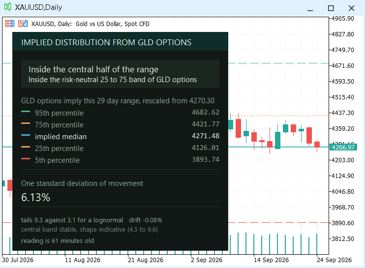
Implied percentile levels and the diagnostics panel drawn on a gold chart
The ladder in the panel reports the five published percentiles mapped onto the local symbol, the anchor they hang from, and the feed's own reliability ranking. The panel states which quantities the feed calls reliable and which it does not, so the caveat travels with the number instead of living only in this article. The screenshots in this section were taken with the revised programs on later readings, so their figures differ from both tables.
The same service reads a different feed and a different symbol when asked to. Nothing in the program is specific to gold.
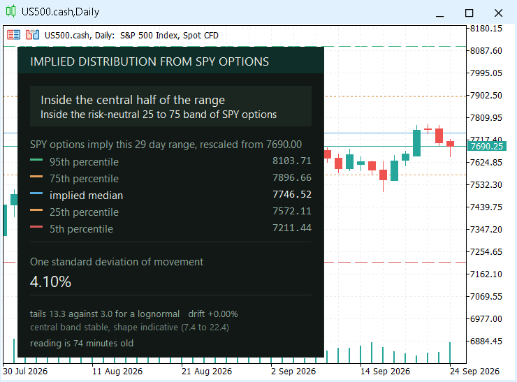
The same service configured for the S&P feed on a US500 chart
The band is visibly narrower here than on gold, which is what the results table already reported: the SPY reading spans 92.3033 to 105.6377 percent of its forward against 88.8141 to 112.4808 for GLD. The picture is a later reading than the table, and the ordering is the same.
The design decision that took longest to get right is not visible in either screenshot. A distribution answers the question of where price can finish, starting from here, and "here" has to be a fixed point. My first version recomputed the levels from the latest price on every cycle. The levels looked correct, the panel looked correct, and the whole thing was useless. The band followed the price, so price sat in the middle of it permanently, and the tail alert could never fire. You cannot leave a band that moves with you.
So the anchor is fixed. The price the band hangs from is recorded once per feed symbol, local symbol, and expiry in a terminal global variable, which survives restarts, and the anchor stays put until the expiry rolls over. The band edges are the anchor multiplied by the published ratios, so they still move when the options reprice, but they no longer move with the local price.

Startup push confirming that notifications reach the phone
That is the startup push, not an alert. It exists because a monitor whose notifications silently fail is worse than no monitor: you would believe you were being watched. Sending one message at startup proves the MetaQuotes ID, the terminal setting, and the phone are all working before anything depends on them. The tail alert itself carries more: the zone, the 5 to 95 band in local prices, and the horizon in days, because an alert that says only "tail" is neither actionable nor verifiable afterward.
One timing detail belongs here rather than in a footnote. The feed is re-read every CheckMinutes, but the local price is re-read on every two-second pass, so the zone on the panel and the band-crossing alert follow the price between feed reads. Only the band itself changes at a feed read.
The alert sits on the 5 and 95 edges, which the sensitivity study ranks as less stable than the central band: across the fifty-four specifications they moved by about 2.5 to 3.3 percent. The alert is therefore a prompt to look, not an event with a known probability. Setting AlertCentral moves it to the 25 and 75 edges, which moved far less.
The four files and what each one does
The system has four source files, which are easiest to understand from the outside in.
implied_density_feed.py is the only piece that touches the options market. It accepts the optionable ETF through "--ticker" and publishes one flat JSON object per run.
ImpliedDensityMonitor.mqh holds CDensityEngine: it fetches the chosen feed, resolves the anchor, maps the relative levels onto LocalSymbol, classifies where price sits, and produces the notification sentence. If you want this inside an indicator or Expert Advisor, this is the reusable file.
ImpliedDensityCheck.mq5 is the flat example script. ImpliedDensityMonitorService.mq5 owns the loop, lines, panel, and alerts, and contains no distribution mathematics of its own.
The split is the point. The mapping lives in one place, so the lines, the panel, and the phone alert cannot disagree with each other.
The density engine class
The class holds its configuration, the published distribution, the levels mapped onto the local symbol, and a few private helpers.
//+------------------------------------------------------------------+
//| ImpliedDensityMonitor.mqh                                        |
//| CDensityEngine reads an option-implied probability distribution  |
//| from a published feed and rescales it onto a related local symbol|
//| Two limits travel with the number: the distribution is           |
//| risk-neutral, so it is what options charge rather than a forecast|
//| and the feed and local symbol need not be equivalent instruments.|
//| The rescaling is a monitoring convenience, not an equivalence.   |
//| Reads only. Never trades.                                        |
//+------------------------------------------------------------------+
#ifndef IMPLIED_DENSITY_MONITOR_MQH
#define IMPLIED_DENSITY_MONITOR_MQH

//--- the anchor of each expiry is remembered here between runs
#define GDEN_ANCHOR_PREFIX "GDEN_ANCHOR_"

//+------------------------------------------------------------------+
//| Where the current price sits inside the implied distribution     |
//+------------------------------------------------------------------+
enum ENUM_DENSITY_ZONE
  {
   ZONE_NONE,          // no usable reading yet
   ZONE_BELOW_TAIL,    // under the 5th percentile
   ZONE_LOWER,         // between the 5th and 25th
   ZONE_CENTRAL,       // between the 25th and 75th
   ZONE_UPPER,         // between the 75th and 95th
   ZONE_ABOVE_TAIL     // above the 95th percentile
  };

//+------------------------------------------------------------------+
//| Option-implied distribution engine                               |
//+------------------------------------------------------------------+
class CDensityEngine
  {
private:
   //--- configuration
   string            m_url;
   string            m_symbol;
   string            m_expectFeed;
   int               m_timeout;
   //--- published distribution, as multiples of the ETF forward
   double            m_forward;
   double            m_spot;
   double            m_r05;
   double            m_r25;
   double            m_r50;
   double            m_r75;
   double            m_r95;
   double            m_probAbove;
   double            m_move1sd;
   double            m_skew;
   double            m_kurt;
   double            m_benchSkew;
   double            m_benchKurt;
   double            m_negMass;
   double            m_sensKurtLo;
   double            m_sensKurtHi;
   int               m_days;
   string            m_expiry;
   string            m_feedSymbol;
   //--- mapped onto the local terminal price
   double            m_price;
   double            m_anchor;
   double            m_level05;
   double            m_level25;
   double            m_level50;
   double            m_level75;
   double            m_level95;
   ENUM_DENSITY_ZONE m_zone;
   //--- housekeeping
   string            m_updated;
   int               m_ageMinutes;
   string            m_lastError;
Its parsing and download helpers come from the script above, moved inside the class, plus one more, JsonHas, which checks that a field exists at all. Two private functions carry the logic of the previous sections. ResolveAnchor reads the anchor from a global variable keyed by feed symbol, local symbol, and expiry, writing it once if absent. Classify decides which part of the distribution the current price occupies.
   //--- the local price the distribution is rescaled from, fixed for the expiry
   //--- A distribution answers "where can price finish, starting from here". If the
   //--- levels were rebuilt around the latest price on every cycle, the band would
   //--- follow price, price would sit in the middle of it forever, and nothing could
   //--- ever be learned from it. So the anchor is set once per expiry and kept.
   //--- The percentile ratios still update with each feed, so the band edges move
   //--- when the options reprice, but they no longer move with the local price.
   double            ResolveAnchor()
     {
      string key = GDEN_ANCHOR_PREFIX + m_feedSymbol + "_" + m_symbol + "_" + m_expiry;
      if(GlobalVariableCheck(key))
        {
         double stored = GlobalVariableGet(key);
         if(stored > 0.0)
            return stored;
        }
      GlobalVariableSet(key, m_price);
      return m_price;
     }

   //--- decide which part of the distribution the current price occupies
   ENUM_DENSITY_ZONE Classify()
     {
      if(m_price <= 0.0)
         return ZONE_NONE;
      if(m_price < m_level05)
         return ZONE_BELOW_TAIL;
      if(m_price < m_level25)
         return ZONE_LOWER;
      if(m_price <= m_level75)
         return ZONE_CENTRAL;
      if(m_price <= m_level95)
         return ZONE_UPPER;
      return ZONE_ABOVE_TAIL;
     }
And the public surface. Configure it, call Compute, then ask for whatever you need. Refresh re-reads the local price and re-classifies it against the levels already held, without downloading anything.
public:
                     CDensityEngine() : m_url(""), m_symbol("XAUUSD"), m_expectFeed(""),
                                        m_timeout(5000), m_forward(0), m_spot(0),
                                        m_r05(0), m_r25(0), m_r50(0), m_r75(0), m_r95(0),
                                        m_probAbove(0), m_move1sd(0), m_skew(0), m_kurt(0),
                                        m_benchSkew(0), m_benchKurt(0),
                                        m_negMass(0), m_sensKurtLo(0), m_sensKurtHi(0),
                                        m_days(0), m_expiry(""), m_feedSymbol(""),
                                        m_price(0), m_anchor(0), m_level05(0), m_level25(0),
                                        m_level50(0), m_level75(0), m_level95(0),
                                        m_zone(ZONE_NONE), m_updated(""),
                                        m_ageMinutes(-1), m_lastError("")
     {
     }

   //--- feed location, the local symbol the distribution is mapped onto, and the
   //--- optionable ETF the feed must describe. An empty expected symbol skips the
   //--- check; a set one catches a FeedURL that points at the wrong instrument
   void              Configure(const string url, const string symbol, const int timeout,
                               const string expectFeed = "")
     {
      m_url = url;
      m_symbol = symbol;
      m_expectFeed = expectFeed;
      m_timeout = (timeout < 1000 ? 1000 : timeout);
     }

   //--- forget the stored anchor, so the next reading starts from today's price
   void              ResetAnchor()
     {
      if(m_expiry == "")
         return;
      string key = GDEN_ANCHOR_PREFIX + m_feedSymbol + "_" + m_symbol + "_" + m_expiry;
      if(GlobalVariableCheck(key))
         GlobalVariableDel(key);
     }

   //--- fetch and map; false means LastError() explains why
   bool              Compute()
     {
      m_lastError = "";
      string json = Download();
      if(json == "")
         return false;

      //--- every field the class reads must be present, not merely non-zero,
      //--- so a truncated or renamed feed is reported by name instead of
      //--- showing a zero that looks like a reading
      string need[] = {"symbol", "expiry", "spot", "forward", "days_to_expiry",
                       "r05", "r25", "r50", "r75", "r95", "updated_utc",
                       "prob_above_spot", "implied_move_1sd_pct", "skewness",
                       "kurtosis", "bench_skewness", "bench_kurtosis",
                       "neg_mass_pct", "sens_kurt_min", "sens_kurt_max"};
      for(int i = 0; i < ArraySize(need); i++)
        {
         if(!JsonHas(json, need[i]))
           {
            m_lastError = "the feed has no " + need[i] + " field";
            return false;
           }
        }
      m_feedSymbol = JsonText(json, "symbol");
      if(m_expectFeed != "" && m_feedSymbol != m_expectFeed)
        {
         m_lastError = "the feed describes " + m_feedSymbol + ", expected " + m_expectFeed;
         return false;
        }

      m_forward = JsonNumber(json, "forward");
      m_spot = JsonNumber(json, "spot");
      m_r05 = JsonNumber(json, "r05");
      m_r25 = JsonNumber(json, "r25");
      m_r50 = JsonNumber(json, "r50");
      m_r75 = JsonNumber(json, "r75");
      m_r95 = JsonNumber(json, "r95");
      if(m_r05 <= 0.0 || m_r95 <= 0.0 || m_r05 >= m_r95 ||
         m_forward <= 0.0 || m_spot <= 0.0)
        {
         m_lastError = "the feed carried no usable distribution";
         return false;
        }

      m_probAbove = JsonNumber(json, "prob_above_spot");
      m_move1sd = JsonNumber(json, "implied_move_1sd_pct");
      m_skew = JsonNumber(json, "skewness");
      m_kurt = JsonNumber(json, "kurtosis");
      m_benchSkew = JsonNumber(json, "bench_skewness");
      m_benchKurt = JsonNumber(json, "bench_kurtosis");
      //--- diagnostics: how much repair the density needed, and how far the
      //--- shape moves under other reasonable specifications of the fit
      m_negMass = JsonNumber(json, "neg_mass_pct");
      m_sensKurtLo = JsonNumber(json, "sens_kurt_min");
      m_sensKurtHi = JsonNumber(json, "sens_kurt_max");
      m_days = (int)JsonNumber(json, "days_to_expiry");
      m_expiry = JsonText(json, "expiry");
      m_updated = JsonText(json, "updated_utc");

      m_price = SymbolInfoDouble(m_symbol, SYMBOL_BID);
      if(m_price <= 0.0)
        {
         m_lastError = "no price for " + m_symbol + ", open its chart once";
         return false;
        }
      //--- The feed publishes percentiles as multiples of the ETF forward, while
      //--- the anchor is a spot-like local price. Multiplying by forward / spot
      //--- first re-expresses each percentile as a multiple of the ETF spot, so
      //--- the ETF's own carry is not mistaken for part of the distribution.
      //--- The local symbol's carry, sessions and funding remain its own
      double scale = m_forward / m_spot;
      //--- the levels hang off the anchor, not off the latest tick
      m_anchor = ResolveAnchor();
      m_level05 = m_anchor * scale * m_r05;
      m_level25 = m_anchor * scale * m_r25;
      m_level50 = m_anchor * scale * m_r50;
      m_level75 = m_anchor * scale * m_r75;
      m_level95 = m_anchor * scale * m_r95;
      m_zone = Classify();

      datetime stamp = FeedTime(m_updated);
      m_ageMinutes = (stamp > 0 ? (int)((TimeGMT() - stamp) / 60) : -1);
      return true;
     }

   //--- re-read the local price and re-classify it against the levels already
   //--- held, without downloading anything. Called on every redraw, so the zone
   //--- and the alert follow the price between feed reads
   bool              Refresh()
     {
      if(m_anchor <= 0.0)
         return false;
      double bid = SymbolInfoDouble(m_symbol, SYMBOL_BID);
      if(bid <= 0.0)
         return false;
      m_price = bid;
      m_zone = Classify();
      return true;
     }
Compute is strict about failure. If the download fails, a required field is missing, the feed describes a different ETF than the one expected, the feed carries no usable distribution, or the terminal has no price for LocalSymbol, it returns false and leaves the reason in LastError, so callers can show the reason instead of presenting a stale reading as current.
   //--- results
   double            Price()      const { return m_price; }        // local price now
   double            Anchor()     const { return m_anchor; }       // price the band hangs from
   double            Level05()    const { return m_level05; }      // 5th percentile
   double            Level25()    const { return m_level25; }      // 25th percentile
   double            Level50()    const { return m_level50; }      // implied median
   double            Level75()    const { return m_level75; }      // 75th percentile
   double            Level95()    const { return m_level95; }      // 95th percentile
   double            ProbAbove()  const { return m_probAbove; }    // 0.5 = even odds
   double            Move1sd()    const { return m_move1sd; }      // percent of forward
   double            Skewness()   const { return m_skew; }         // shape of the density
   double            Kurtosis()   const { return m_kurt; }         // compare with BenchKurt
   double            BenchSkew()  const { return m_benchSkew; }    // lognormal reference
   double            BenchKurt()  const { return m_benchKurt; }    // lognormal reference
   double            NegMass()    const { return m_negMass; }      // percent clipped away
   double            SensKurtLo() const { return m_sensKurtLo; }   // kurtosis across specs
   double            SensKurtHi() const { return m_sensKurtHi; }   // kurtosis across specs
   int               Days()       const { return m_days; }         // days to expiry
   string            Expiry()     const { return m_expiry; }       // expiry read
   string            FeedSymbol() const { return m_feedSymbol; }   // options instrument
   ENUM_DENSITY_ZONE Zone()       const { return m_zone; }         // where price sits
   string            UpdatedUTC() const { return m_updated; }      // feed timestamp
   int               AgeMinutes() const { return m_ageMinutes; }   // -1 when unknown
   string            LastError()  const { return m_lastError; }    // why Compute() failed

   //--- how far price has travelled from the anchor, in percent
   double            DriftPct()
     {
      if(m_anchor <= 0.0)
         return 0.0;
      return 100.0 * (m_price - m_anchor) / m_anchor;
     }

   //--- headline for the panel, in words
   string            ZoneHeadline()
     {
      switch(m_zone)
        {
         case ZONE_BELOW_TAIL:
            return "Below the implied 5 percent tail";
         case ZONE_LOWER:
            return "In the lower quarter of the range";
         case ZONE_CENTRAL:
            return "Inside the central half of the range";
         case ZONE_UPPER:
            return "In the upper quarter of the range";
         case ZONE_ABOVE_TAIL:
            return "Above the implied 95 percent tail";
         default:
            return "No reading";
        }
     }

   //--- the second line, explaining the headline
   string            ZoneExplain()
     {
      switch(m_zone)
        {
         case ZONE_BELOW_TAIL:
         case ZONE_ABOVE_TAIL:
            return StringFormat("Outside the risk-neutral 5 to 95 band of %s options",
                                m_feedSymbol);
         case ZONE_LOWER:
         case ZONE_UPPER:
            return "Inside the 5 to 95 band, outside the 25 to 75";
         case ZONE_CENTRAL:
            return StringFormat("Inside the risk-neutral 25 to 75 band of %s options",
                                m_feedSymbol);
         default:
            return "Waiting for the feed";
        }
     }

   //--- true when the price sits outside the 5 to 95 band
   bool              InTail()
     {
      return (m_zone == ZONE_BELOW_TAIL || m_zone == ZONE_ABOVE_TAIL);
     }

   //--- true when the price sits outside the 25 to 75 band, the more stable
   //--- edges, for callers that prefer to alert on those
   bool              OutsideCentral()
     {
      return (m_zone != ZONE_NONE && m_zone != ZONE_CENTRAL);
     }

   //--- one plain sentence, short enough for a push notification
   string            Summary()
     {
      return StringFormat("%s. From %.0f, %s options implied a risk-neutral %d day 5 to 95 band of %.0f to %.0f, and %s is at %.0f.",
                          ZoneHeadline(), m_anchor, m_feedSymbol, m_days, m_level05,
                          m_level95, m_symbol, m_price);
     }
  };

#endif // IMPLIED_DENSITY_MONITOR_MQH
//+------------------------------------------------------------------+
Drawing the levels from a service
One line makes this a service rather than a script, and one property of MQL5 objects makes a service able to draw at all.
//+------------------------------------------------------------------+
//| ImpliedDensityMonitorService.mq5                                 |
//| MetaTrader 5 service. Runs in the background with no chart of    |
//| its own, reads the option-implied probability distribution of    |
//| an optionable ETF, rescales its percentile levels onto a related |
//| local symbol, draws them on an open chart, keeps a panel current,|
//| and sends a push notification when price leaves the risk-neutral |
//| 5 to 95 band of those options. The mapping is a monitoring       |
//| convenience, not an equivalence between instruments.             |
//| Reads only. Never trades.                                        |
//+------------------------------------------------------------------+
#property service
#property version   "2.10"
#property description "Background monitor: option-implied distribution, chart levels and tail alerts."

#include "ImpliedDensityMonitor.mqh"

//--- feed and measurement
input string          FeedURL       = "https://raw.githubusercontent.com/GeneTheStoic/gold-density-feed/main/feed_gld.json"; // implied distribution feed
input string          LocalSymbol   = "XAUUSD";    // matching symbol in Market Watch
input string          FeedSymbol    = "GLD";       // ETF the feed must describe ("" = no check)
input int             TimeoutMs     = 5000;        // web request timeout
//--- monitoring
input int             CheckMinutes  = 15;          // how often to re-read the feed
//--- an option chain does not update overnight or on weekends, so a reading can be
//--- legitimately old without being wrong. 900 minutes covers the normal pause
input int             StaleMinutes  = 900;         // warn when the feed is older than this
//--- drawing
input bool            ShowLevels    = true;        // draw the percentile lines on the chart
input bool            ShowPanel     = true;        // draw the panel
input string          PanelSymbol   = "";          // chart to draw on ("" = the LocalSymbol chart)
input int             PanelX        = 20;          // panel x
input int             PanelY        = 30;          // panel y
input double          UIScale       = 1.0;         // interface scale
//--- alerts
input bool            AlertOnTail   = true;        // push when price leaves the 5 to 95 band
//--- the 5 and 95 edges are the least stable output of the recovery, so the
//--- alert can be moved to the 25 and 75 edges, which move far less
input bool            AlertCentral  = false;       // alert on the 25 to 75 band instead
input int             CooldownMinutes = 60;        // minimum minutes between repeat pushes
input bool            StartupPush   = true;        // send a test push on start
input bool            ResetAnchor   = false;       // forget the stored anchor and start from today

//--- panel palette
#define CBG      C'18,24,21'
#define CBORD    C'34,48,41'
#define CHEAD    C'15,46,42'
#define CINK     C'232,240,234'
#define CMUT     C'140,166,154'
#define CKICK    C'111,131,120'
#define CTRACK   C'28,38,32'
#define CGREEN   C'52,201,138'
#define CAMBER   C'230,184,75'
#define CRED     C'229,86,86'
#define CFILLG   C'28,56,46'
#define CFILLA   C'58,50,26'
#define CFILLR   C'58,32,32'
//--- the five level colors, shared by the lines and the ladder swatches
#define CL_TAIL_LO   C'214,90,90'
#define CL_QUART_LO  C'226,160,92'
#define CL_MEDIAN    C'86,170,222'
#define CL_QUART_HI  C'226,160,92'
#define CL_TAIL_HI   C'70,186,132'
#define PFX      "GDEN_"
#define UIF      "Segoe UI"
#define MONO     "Consolas"
A service has no chart of its own, but it can draw on any open chart, because every object function in MQL5 takes a chart identifier as its first argument. Indicators pass zero, meaning "my own chart"; a service passes the identifier of a chart it found with ChartFirst and ChartNext. That detail is what lets a background program keep live levels in front of you.
//--- DPI scaling
double gScl = 1.0, gFscl = 1.0;
//+------------------------------------------------------------------+
//| Scale a distance by the DPI factor                               |
//+------------------------------------------------------------------+
int S(double v) { return (int)MathRound(v * gScl); }
//+------------------------------------------------------------------+
//| Scale a font size by the UI scale factor                         |
//+------------------------------------------------------------------+
int FS(int p) { int f = (int)MathRound(p * gFscl); return (f < 6 ? 6 : f); }
//+------------------------------------------------------------------+
//| Colour of one percentile level, by index from the low tail up    |
//+------------------------------------------------------------------+
color LevelColor(const int which)
  {
   switch(which)
     {
      case 0:
         return CL_TAIL_LO;
      case 1:
         return CL_QUART_LO;
      case 2:
         return CL_MEDIAN;
      case 3:
         return CL_QUART_HI;
      default:
         return CL_TAIL_HI;
     }
  }
Beneath those sit four short wrappers around ObjectCreate and ObjectSetInteger, one each for creating a rectangle, positioning it, writing a label, and hiding a label. All four are conventional, and all four are in the attached file.
The lines themselves carry no text. An earlier version labeled each one on the chart, and the labels drifted into the price scale as soon as anything was scrolled or zoomed. Every number lives in the panel instead, as a ladder of five rows: a color swatch matching the line, the name of the percentile, and the price, right-aligned in a monospaced font so the digits line up.
//+------------------------------------------------------------------+
//| Draw or update one horizontal level line                         |
//+------------------------------------------------------------------+
void DrawLine(long id, string n, double price, color clr, int style)
  {
   string nm = PFX + n;
   if(ObjectFind(id, nm) < 0)
      ObjectCreate(id, nm, OBJ_HLINE, 0, 0, price);
   ObjectSetDouble(id, nm, OBJPROP_PRICE, price);
   ObjectSetInteger(id, nm, OBJPROP_COLOR, clr);
   ObjectSetInteger(id, nm, OBJPROP_STYLE, style);
   ObjectSetInteger(id, nm, OBJPROP_WIDTH, 1);
   ObjectSetInteger(id, nm, OBJPROP_BACK, true);
   ObjectSetInteger(id, nm, OBJPROP_SELECTABLE, false);
   ObjectSetInteger(id, nm, OBJPROP_HIDDEN, true);
   ObjectSetString(id, nm, OBJPROP_TOOLTIP, n);
  }
//+------------------------------------------------------------------+
//| Draw the five percentile lines. The numbers live in the panel,   |
//| so nothing is written on the chart itself and nothing collides.  |
//+------------------------------------------------------------------+
void DrawLevels(long id, CDensityEngine &eng)
  {
   double prices[5];
   prices[0] = eng.Level05();
   prices[1] = eng.Level25();
   prices[2] = eng.Level50();
   prices[3] = eng.Level75();
   prices[4] = eng.Level95();
   string names[] = {"l05", "l25", "l50", "l75", "l95"};
   for(int i = 0; i < 5; i++)
     {
      int style = (i == 2 ? STYLE_SOLID : (i == 0 || i == 4 ? STYLE_DASH : STYLE_DOT));
      DrawLine(id, names[i], prices[i], LevelColor(i), style);
     }
  }
//+------------------------------------------------------------------+
//| Remove the level lines from the chart                            |
//+------------------------------------------------------------------+
void ClearLevels(long id)
  {
   string names[] = {"l05", "l25", "l50", "l75", "l95"};
   for(int i = 0; i < ArraySize(names); i++)
     {
      string nm = PFX + names[i];
      if(ObjectFind(id, nm) >= 0)
         ObjectDelete(id, nm);
     }
  }
//+------------------------------------------------------------------+
//| Color matching where the price sits in the distribution          |
//+------------------------------------------------------------------+
color ZoneColor(const ENUM_DENSITY_ZONE zone)
  {
   switch(zone)
     {
      case ZONE_BELOW_TAIL:
         return CRED;
      case ZONE_ABOVE_TAIL:
         return CGREEN;
      case ZONE_LOWER:
      case ZONE_UPPER:
         return CAMBER;
      case ZONE_CENTRAL:
         return CINK;
      default:
         return CMUT;
     }
  }
//+------------------------------------------------------------------+
//| Band fill matching where the price sits                          |
//+------------------------------------------------------------------+
color ZoneFill(const ENUM_DENSITY_ZONE zone)
  {
   switch(zone)
     {
      case ZONE_BELOW_TAIL:
         return CFILLR;
      case ZONE_ABOVE_TAIL:
         return CFILLG;
      case ZONE_LOWER:
      case ZONE_UPPER:
         return CFILLA;
      default:
         return CTRACK;
     }
  }
//+------------------------------------------------------------------+
//| Find the chart to draw on                                        |
//+------------------------------------------------------------------+
long FindChart()
  {
//--- the levels are prices of LocalSymbol, so by default they belong on that
//--- symbol's chart and nowhere else. Drawing them on an unrelated chart would
//--- show plausible lines at meaningless prices, so nothing is drawn instead
   static bool warned = false;
   string want = (PanelSymbol == "" ? LocalSymbol : PanelSymbol);
   long id = ChartFirst();
   while(id >= 0)
     {
      if(ChartSymbol(id) == want)
        {
         warned = false;
         return id;
        }
      id = ChartNext(id);
     }
   if(!warned)
      Print("No ", want, " chart is open. Open one and the levels will appear on it.");
   warned = true;
   return -1;
  }
//+------------------------------------------------------------------+
//| One row of the levels ladder: swatch, label, price               |
//+------------------------------------------------------------------+
void LadderRow(long id, string n, int x, int y, int colW, int which,
               string tag, double price, int digits, bool here)
  {
   color clr = LevelColor(which);
   setRect(id, n + "_sw", x, y + S(5), S(14), S(2), clr);
   L(id, n + "_k", x + S(22), y, tag, (here ? CINK : CMUT), FS(9), UIF);
   L(id, n + "_v", x + colW, y, DoubleToString(price, digits),
     (here ? CINK : CMUT), FS(9), MONO, ANCHOR_RIGHT_UPPER);
  }
The panel itself is coordinate arithmetic and nothing more, laid out from the top down so that adding a row never disturbs the rows above it. It puts the meaning first and the mathematics second: the headline in words, then the ladder, then the implied move, then the shape of the distribution and the age of the reading.
//+------------------------------------------------------------------+
//| Draw the panel on the given chart                                |
//+------------------------------------------------------------------+
void DrawPanel(long id, CDensityEngine &eng, bool hasData)
  {
   int PX = PanelX, PY = PanelY;
//--- the column has to hold the longest line in the panel, which is the ladder
//--- caption naming the rescaling anchor, not the header
   int pad = S(14), colW = S(322);
   int Wpx = pad + colW + pad;
   int hdH = S(30);
   string rows[] = {"r95", "r75", "r50", "r25", "r05"};
   setRect(id, "bg", PX, PY, Wpx, hdH + S(40), CBG, CBORD);
   setRect(id, "hd", PX, PY, Wpx, hdH, CHEAD);
   string panelTitle = (hasData
                        ? StringFormat("IMPLIED DISTRIBUTION FROM %s OPTIONS",
                                       eng.FeedSymbol())
                        : "IMPLIED DISTRIBUTION MONITOR");
   L(id, "title", PX + pad, PY + S(7), panelTitle, CINK, FS(10), UIF);
   if(!hasData)
     {
      hideL(id, "head");
      hideL(id, "headsub");
      hideL(id, "mv_k");
      hideL(id, "mv_v");
      hideL(id, "shape");
      hideL(id, "caveat");
      hideL(id, "age");
      hideL(id, "ladder_k");
      for(int i = 0; i < ArraySize(rows); i++)
        {
         hideL(id, rows[i] + "_k");
         hideL(id, rows[i] + "_v");
        }
      L(id, "empty", PX + pad, PY + hdH + S(12), "Waiting for the distribution feed", CINK, FS(9), UIF);
      L(id, "empty2", PX + pad, PY + hdH + S(30), eng.LastError(), CMUT, FS(8), UIF);
      setRect(id, "bg", PX, PY, Wpx, hdH + S(52), CBG, CBORD);
      ChartRedraw(id);
      return;
     }
   hideL(id, "empty");
   hideL(id, "empty2");
   int y = PY + hdH + S(14);
   int xL = PX + pad;
   color zc = ZoneColor(eng.Zone());
   int digits = (int)SymbolInfoInteger(LocalSymbol, SYMBOL_DIGITS);
//--- headline band: where price sits inside the implied distribution
   int heroH = S(46);
   setRect(id, "hero_tk", xL, y, colW, heroH, CTRACK);
   double span = eng.Level95() - eng.Level05();
   double fill = (span > 0.0 ? (eng.Price() - eng.Level05()) / span : 0.5);
   if(fill < 0.05)
      fill = 0.05;
   if(fill > 1.0)
      fill = 1.0;
   setRect(id, "hero_fl", xL, y, (int)MathMax(S(3), colW * fill), heroH, ZoneFill(eng.Zone()));
   L(id, "head", xL + S(12), y + S(15), eng.ZoneHeadline(), CINK, FS(10), UIF, ANCHOR_LEFT);
   L(id, "headsub", xL + S(12), y + S(32), eng.ZoneExplain(), zc, FS(9), UIF, ANCHOR_LEFT);
   y += heroH + S(12);
//--- the ladder: every line on the chart, named and priced
   L(id, "ladder_k", xL, y,
     StringFormat("%s options imply this %d day range, rescaled from %s",
                  eng.FeedSymbol(), eng.Days(), DoubleToString(eng.Anchor(), digits)),
     CMUT, FS(9), UIF);
   y += S(20);
   double prices[5];
   prices[0] = eng.Level95();
   prices[1] = eng.Level75();
   prices[2] = eng.Level50();
   prices[3] = eng.Level25();
   prices[4] = eng.Level05();
   string tags[] = {"95th percentile", "75th percentile", "implied median",
                    "25th percentile", "5th percentile"};
   int which[] = {4, 3, 2, 1, 0};
   for(int i = 0; i < 5; i++)
     {
      bool here = (i == 2);
      LadderRow(id, rows[i], xL, y, colW, which[i], tags[i], prices[i], digits, here);
      y += S(19);
     }
   y += S(4);
   setRect(id, "d1", xL, y, colW, S(1), CBORD);
   y += S(14);
//--- the implied move itself
   L(id, "mv_k", xL, y, "One standard deviation of movement", CMUT, FS(9), UIF);
   y += S(18);
   L(id, "mv_v", xL, y, StringFormat("%.2f%%", eng.Move1sd()), CINK, FS(13), UIF);
   y += S(28);
   setRect(id, "d2", xL, y, colW, S(1), CBORD);
   y += S(14);
//--- the shape of the distribution, and how fresh the reading is
   L(id, "shape", xL, y,
     StringFormat("tails %.1f against %.1f for a lognormal   drift %+.2f%%",
                  eng.Kurtosis(), eng.BenchKurt(), eng.DriftPct()),
     CMUT, FS(8), UIF);
   y += S(15);
//--- the band is stable across specifications and the shape is not, so the panel
//--- says so rather than letting the reader treat both as equally solid
   L(id, "caveat", xL, y,
     StringFormat("central band stable, shape indicative (%.1f to %.1f)",
                  eng.SensKurtLo(), eng.SensKurtHi()), CKICK, FS(8), UIF);
   y += S(18);
   int age = eng.AgeMinutes();
   bool stale = (age < 0 || age > StaleMinutes);
   string unit = (age == 1 ? "minute" : "minutes");
   string ageText = (age < 0 ? "reading age unknown"
                    : (stale ? StringFormat("STALE: reading is %d %s old, treat with caution", age, unit)
                             : StringFormat("reading is %d %s old", age, unit)));
   L(id, "age", xL, y, ageText, (stale ? CAMBER : CMUT), FS(8), UIF);
   y += S(24);
   int H = (y - PY);
   setRect(id, "bg", PX, PY, Wpx, H, CBG, CBORD);
   setRect(id, "hd", PX, PY, Wpx, hdH, CHEAD);
   ChartRedraw(id);
  }
And the loop. The feed is re-read on the configured interval while the drawing is refreshed every two seconds, because those are two different problems: the distribution changes slowly, and the price does not. Charts can be closed while a service is running, so each cycle checks that the chart still exists, and the service removes its own objects when it stops.
//+------------------------------------------------------------------+
//| Service program start function                                   |
//+------------------------------------------------------------------+
void OnStart()
  {
//--- DPI scaling for the panel
   double dpi = (double)TerminalInfoInteger(TERMINAL_SCREEN_DPI);
   if(dpi <= 0)
      dpi = 96;
   gScl = (dpi / 96.0) * (UIScale > 0 ? UIScale : 1.0);
   gFscl = (UIScale > 0 ? UIScale : 1.0);
//--- make sure pushes can actually reach the phone
   if(!TerminalInfoInteger(TERMINAL_NOTIFICATIONS_ENABLED))
      Print("Push notifications are DISABLED. Enable them in Tools -> Options -> ",
            "Notifications and enter your MetaQuotes ID, or no alert will arrive.");
   else
      if(StartupPush)
        {
         if(SendNotification("Implied distribution monitor started. You will get an alert when price leaves the monitored band."))
            Print("Startup push sent. Check your phone.");
         else
            Print("Startup push FAILED, error ", GetLastError(),
                  ". Check your MetaQuotes ID in Tools -> Options -> Notifications.");
        }
   CDensityEngine engine;
   engine.Configure(FeedURL, LocalSymbol, TimeoutMs, FeedSymbol);
   bool wasInTail = false;
   bool first = true;
   bool ok = false;
   datetime lastAlert = 0;
   datetime lastFetch = 0;
   long chart = -1;
   int fetchSec = (CheckMinutes < 1 ? 1 : CheckMinutes) * 60;
//--- a failed reading waits this long instead of the full interval, so a
//--- temporary outage recovers quickly. The wait is never zero, because the
//--- redraw loop turns every two seconds and an unguarded retry would ask the
//--- feed host thirty times a minute for as long as the failure lasts
   int retrySec = 60;
   Print("Implied distribution monitor running. Reading the feed every ",
         CheckMinutes, " minutes.");
//--- every clock below is TimeGMT. Server time stops when the market closes,
//--- so a schedule or cooldown measured against it would freeze on weekends
   while(!IsStopped())
     {
      //--- the feed is slow moving, so it is re-read on the configured interval
      long waited = (long)TimeGMT() - (long)lastFetch;
      if(lastFetch == 0 || waited >= (long)(ok ? fetchSec : retrySec))
        {
         ok = (TerminalInfoInteger(TERMINAL_CONNECTED) && engine.Compute());
         if(ok && first && ResetAnchor)
           {
            //--- drop the stored anchor, then read once more so the band hangs
            //--- from today's price instead of the one saved earlier
            engine.ResetAnchor();
            ok = engine.Compute();
            Print("Anchor reset. The band now hangs from ",
                  DoubleToString(engine.Anchor(), 2), ".");
           }
         lastFetch = TimeGMT();
         if(!ok && engine.LastError() != "")
            Print("Reading failed: ", engine.LastError());
        }
      //--- between feed reads the price is re-read and re-classified on every
      //--- pass, so the zone and the alert follow the price within two seconds
      if(ok)
         engine.Refresh();
      //--- the drawing is refreshed every couple of seconds as well, so the panel
      //--- and the lines keep up with scrolling, zooming and a moving price
      if(chart < 0 || ChartPeriod(chart) == 0)
         chart = FindChart();
      if(chart >= 0)
        {
         if(ShowLevels && ok)
            DrawLevels(chart, engine);
         if(ShowPanel)
            DrawPanel(chart, engine, ok);
        }
      if(ok)
        {
         bool inTail = (AlertCentral ? engine.OutsideCentral() : engine.InTail());
         bool changed = (inTail != wasInTail && !first);
         bool cooled = ((long)TimeGMT() - (long)lastAlert >= (long)CooldownMinutes * 60);
         //--- notify only when price crosses out of the monitored band
         if(AlertOnTail && changed && inTail && cooled)
           {
            string msg = "IMPLIED DISTRIBUTION: " + engine.Summary();
            if(SendNotification(msg))
               lastAlert = TimeGMT();
            else
               Print("Push failed, error ", GetLastError());
            Print(msg);
           }
         if(changed || first)
            Print("Zone: ", engine.ZoneHeadline(), " (", engine.Summary(), ")");
         if(first)
            Print("Anchor for expiry ", engine.Expiry(), " is ",
                  DoubleToString(engine.Anchor(), 2),
                  ". It stays fixed until the expiry rolls; the band edges update with each feed.");
         wasInTail = inTail;
         first = false;
        }
      Sleep(2000);
     }
//--- clean the drawing off the chart when the service stops
   if(chart >= 0 && ChartPeriod(chart) > 0)
     {
      ClearLevels(chart);
      ObjectsDeleteAll(chart, PFX);
      ChartRedraw(chart);
     }
   Print("Implied distribution monitor stopped.");
  }
//+------------------------------------------------------------------+
Put ImpliedDensityMonitorService.mq5 and ImpliedDensityMonitor.mqh together in MQL5\Services\ImpliedDensityMonitor\, or unpack the attached archive into the terminal data folder. Compile with F7, then find Services at the bottom of the Navigator, right-click, choose "Add Service," and select it. For notifications, add your MetaQuotes ID under Tools, Options, Notifications. ResetAnchor takes effect on the first successful read after the service starts, because the anchor is keyed by the expiry the feed reports. If the feed is unreachable at startup, the old anchor stays until it can be read.
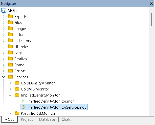
The service in the Navigator.
The service and the class sit in the same folder. That is not tidiness; it is what makes the quoted include path resolve; separating them is the most common reason this build fails to compile for someone else.
FeedURL and LocalSymbol are set as a matched pair, with FeedSymbol naming the ETF in the feed, and those three inputs are the only thing that makes an instance instrument-specific:
| Instrument | FeedURL ends with | LocalSymbol |
|---|---|---|
| Gold | feed_gld.json | XAUUSD |
| Silver | feed_slv.json | XAGUSD |
| S&P 500 | feed_spy.json | US500 |
| Crude oil | feed_uso.json | USOIL |
Add the service once per pair to monitor several instruments at the same time. Use your broker's own symbol names, which vary. The service checks half of that pairing. Set FeedSymbol to the ETF in the file name, GLD, SLV, SPY, or USO, and a feed for any other ETF is refused with a message. It cannot check that LocalSymbol is the market you meant, because broker symbol names vary, so that half stays with you. The levels are drawn only on the LocalSymbol chart; if that chart is not open, nothing is drawn.
Applications in expected range, stops, and position sizing
A measurement is only worth taking if it changes a decision.
The most direct use is the expected range. Most retail range estimates come from ATR or from a multiple of historical volatility, and both are backward-looking by construction. The 25th and 75th percentile levels are a forward-looking, risk-neutral alternative, and they are asymmetric when the market thinks they should be, which no symmetric multiple of a historical number can be.
Stops need more care. The percentiles describe where the ETF may finish at expiry under the risk-neutral measure, while a stop is hit if price touches it at any time before then. Under a driftless random walk the chance of touching a level before expiry is about twice the chance of finishing beyond it. So a percentile marks a finishing level, not a stop-out probability, and it describes the ETF rather than the local symbol.
Position sizing is where the gap between the two volatility numbers becomes practical. On the GLD reading the recovered standard deviation is 7.7759 percent of the forward while the flat-smile Black-76 figure built from the at-the-money volatility alone is 7.1989 percent, about seven percent narrower. If your sizing model runs on a one-standard-deviation move computed from at-the-money implied volatility, it is working with the narrower of two numbers the same chain produces. Neither is wrong, but they answer different questions, and sizing is a question about the wings.
The limits stay where they were: these are an ETF's risk-neutral percentiles rescaled onto your local symbol rather than that symbol's own, the reading says nothing about direction, it describes one expiry, and a distribution that looks calm can be repriced in an afternoon.
For a developer, the useful part may not be any of these instruments. Compute what the terminal cannot compute outside it, publish the result as a small flat JSON file per instrument, read it with WebRequest, and consume it in a service. The distribution is the example; the bridge is the technique.
Conclusion
The path from an option chain to a probability level on a chart is short in outline and long in the details that matter. Read the forward out of put-call parity, solve implied volatility across the strikes in Black-76, smooth the result, reprice a dense grid, difference it twice, check the curve for arbitrage, and normalize. The identity behind it dates from 1978. The first version of this script was about two hundred lines, and most of what has been added since is not mathematics; it is checking: the diagnostics, the sensitivity study, and the tests that say when the answer should be distrusted. The plumbing, again, is a URL.
The result is not a forecast or a native CFD distribution. It is a risk-neutral ETF distribution mapped onto a related chart as a monitoring convenience. GLD, SLV, SPY, and USO all produced usable densities under the same mathematics on two separate afternoons and ranked the same way by band width both times. Two afternoons are a consistency check, not a demonstration that the recovery is stable over time. Their data quality and proxy strength differed, and the quality of a given chain was not stable from one day to the next. The median and interquartile band are the more robust outputs; the outer tails and shape moments are less stable. The median is stable to two tenths of a percent across the sensitivity study, which makes it the most dependable number the pipeline publishes, though stability is not the same as trading value. The kurtosis is not, so it is not quoted to two decimals.
The diagnostics keep that distinction visible, and the second afternoon is the argument for them: the same instrument produced almost the same percentiles from a noticeably worse fit, and only the published counts revealed it. That distinction is the useful part, and it is what the panel repeats every two seconds on the chart.
Background and sources
The identity at the center of this build is Breeden and Litzenberger's, published in 1978, which showed that the second derivative of a call price with respect to strike recovers the price of a state-contingent claim, and therefore the density. [1] Jackwerth and Rubinstein put the method to work on index options and documented how far the recovered distributions depart from lognormality. [2] Bliss and Panigirtzoglou measured the wedge between the risk-neutral distribution and the real-world one, which is the formal version of the caveat above. [3] Figlewski's treatment is the most practical account of the estimation problems, particularly in the tails [4], and Malz gives a reproducible recipe for the smoothing step. [5] The inversion itself goes back to Black and Scholes in 1973 [6], in the forward-based form Black published three years later. [7]
The framing here follows the options and volatility theory I studied at Nicolaus Copernicus University. If you read one of these, read Figlewski, which is honest about how much of the answer depends on decisions the mathematics does not make for you.
References
[1] Breeden, D. and Litzenberger, R. (1978). Prices of State-Contingent Claims Implicit in Option Prices. The Journal of Business, 51(4), 621 to 651. https://doi.org/10.1086/296025
[2] Jackwerth, J. and Rubinstein, M. (1996). Recovering Probability Distributions from Option Prices. The Journal of Finance, 51(5), 1611 to 1631. https://doi.org/10.1111/j.1540-6261.1996.tb05219.x
[3] Bliss, R. and Panigirtzoglou, N. (2004). Option-Implied Risk Aversion Estimates. The Journal of Finance, 59(1), 407 to 446. https://doi.org/10.1111/j.1540-6261.2004.00637.x
[4] Figlewski, S. (2010). Estimating the Implied Risk-Neutral Density for the U.S. Market Portfolio. In: Volatility and Time Series Econometrics: Essays in Honor of Robert F. Engle. Oxford University Press, 323 to 353. https://doi.org/10.1093/acprof:oso/9780199549498.003.0015
[5] Malz, A. (2014). A Simple and Reliable Way to Compute Option-Based Risk-Neutral Distributions. Federal Reserve Bank of New York Staff Reports, No. 677. https://www.newyorkfed.org/research/staff_reports/sr677.html
[6] Black, F. and Scholes, M. (1973). The Pricing of Options and Corporate Liabilities. Journal of Political Economy, 81(3), 637 to 654. https://doi.org/10.1086/260062
[7] Black, F. (1976). The Pricing of Commodity Contracts. Journal of Financial Economics, 3(1-2), 167 to 179. https://doi.org/10.1016/0304-405X(76)90024-6
Files used in the article
| # | Name | Type | Description |
|---|---|---|---|
| 1 | implied_density_feed.py | Python script | Accepts an ETF ticker, recovers its risk-neutral density, and publishes one flat JSON feed |
| 2 | ImpliedDensityMonitor.mqh | Class library | Reads one feed, resolves the anchor, maps percentiles onto LocalSymbol, and classifies price |
| 3 | ImpliedDensityCheck.mq5 | Script | Fetches one feed and prints the mapped percentile levels |
| 4 | ImpliedDensityMonitorService.mq5 | Service | Draws levels and a panel and sends notifications when price leaves the risk-neutral 5 to 95 percent band |
| 5 | MQL5.zip | Archive | Mirrors the Scripts and Services project folders for direct installation |
Warning: All rights to these materials are reserved by MetaQuotes Ltd. Copying or reprinting of these materials in whole or in part is prohibited.
This article was written by a user of the site and reflects their personal views. MetaQuotes Ltd is not responsible for the accuracy of the information presented, nor for any consequences resulting from the use of the solutions, strategies or recommendations described.

 How to Detect and Normalize Chart Objects in MQL5 (Part 6): Manipulating Chart Objects with MetaTrader 5 Agentic AI Assistant
 Implementing an LLM Agent with SQL Memory in MetaTrader 5
 Features of Experts Advisors
 Uncertainty as a Model (Part 4): Random Processes — The Dynamics of Uncertainty

- Free trading apps
- Over 8,000 signals for copying
- Economic news for exploring financial markets
You agree to website policy and terms of use