Defining your Edge (Part 4): Applying Isotonic Regression and PNN Price-Forecasting in an Expert Advisor

Introduction

We continue this series on Developing-Your-Edge where another article, following this-one, means we have a new algorithm-network pairing. The importance of an Edge can be very subjective with some traders preferring to follow macro trends and popular entry signals. These can work well in trending environments, however the case can be made that if one is to be a trader for a reasonable amount of time, he needs to develop or be familiar with a unique perspective of the markets that leads him to engage a specific toolset. This would not have him miss out on the macro trends and "upside", but more importantly it would leave him relatively protected when markets face a "correction".  In using algorithms we always need some typical indicator and for this article we are looking at oscillators.

Oscillators are usually presented as holistic trading tools: When the RSI gets to an extreme, or if the Stochastic presents a cross, the trader acts. When using automated systems though processing these patterns to determine whether they deserve an entry is not as easy as it may seem initially. The RSI could be bullish at 65 in one context and overbought in another, while a Stochastic crossover can mark either transition or noise. In these situations, neither indicator quantifies how much confidence to attach to the signal.

Thus, the custom signal that we examine in this article treats this as a calibration problem. We engage seven interpretations of RSI, Stochastic, and some price action to initially generate a bounded directional score. Isotonic Regression then maps that score onto an empirically ordered probability. An alternative Probability based Neural Network poses the question of whether the current multidimensional state looks like past bullish or bearish states.

The separation of labor is very simple: the isotonic regression tests if stronger raw signals are worth increasingly more confidence; the PNN evaluates if the internal composition of a signal looks like historic useful cases. More layers tend to imply more ways of overfitting; therefore, our goal here leans towards rapid proofing instead of "proof of superiority".

MQL5 Implementation

Our custom-built signal class 'CSignalIsotonicPNN' inherits from 'CExpertSignal' and flows its decisions through the Wizard-facing 'LongCondition()' and 'ShortCondition()' methods. The input parameter 'm_signal_mode' chooses what market behavior is being interpreted, while the parameter 'm_model_mode' picks how that interpretation gets translated into a probability. The rest of the inputs cover RSI and Stochastic settings via 'PatternLookback'; isotonic controls through 'CalibrationWindow' and 'ForecastHorizon', and PNN controls that include 'PNNSamples', 'PNNSigma', as well as 'PNNWeight'.

This setting apart allows us to hold Momentum Agreement constant while comparing isotonic-only with isotonic and PNN, or to keep the model unchanged while alternating among the seven algorithm modes. It also affords us a wider degree of optimization. Rapid proofing therefore helps separate assumptions instead of searching continuously for the most profitable parameter combination.

One Scale for Seven Interpretations

The seven modes of the isotonic algorithm all use the same source information. RSI, Stochastic, and some price-context measurements. Every one of them returns a score in the range [0,1] with a value of 0.5 implying neutrality. We take scores over 0.5 to signify bullish outlook while those below are bearish. With that said, this score is not yet a probability. A value of say 0.75 would only mean that our algorithm found some relatively strong bullish evidence. When using 'ModelMode=0', isotonic regression alone calibrates this score.

   //--- selected raw pattern score in [0,1], where 0.5 is neutral
   double             ModeScore(int ind);

   //--- seven independently coded signal modes
   double             Mode0MomentumAgreement(int ind);
   double             Mode1ExtremeReversal(int ind);
   double             Mode2ZoneCross(int ind);
   double             Mode3CenterlineImpulse(int ind);
   double             Mode4Divergence(int ind);
   double             Mode5PullbackContinuation(int ind);
   double             Mode6BreakoutConfirmation(int ind);

   //--- isotonic regression
   bool               BuildCalibrationSet(int ind,double &x[],double &y[],int &count);
   void               SortPairs(double &x[],double &y[],int count);
   double             IsotonicProbability(int ind,double raw_score);

   //--- probabilistic neural network
   bool               FeatureVector(int ind,double &features[]);
   double             PNNProbability(int ind);

   //--- complete model
   double             ProbabilityUp(int ind);
  };

In 'ModelMode=1' though, the calibrated result gets blended with a PNN posterior. Our exploration focus therefore narrows down to: "given the same raw mode, does the PNN add anything besides isotonic calibration"?

Initialization

//+------------------------------------------------------------------+
//| Validation settings protected data.                              |
//+------------------------------------------------------------------+
bool CSignalIsotonicPNN::ValidationSettings(void)
  {
//--- validation settings of additional filters
   if(!CExpertSignal::ValidationSettings())
      return(false);

   if(m_model_mode<0 || m_model_mode>1)
     {
      printf(__FUNCTION__+": ModelMode must be 0 or 1");
      return(false);
     }
   if(m_signal_mode<0 || m_signal_mode>6)
     {
      printf(__FUNCTION__+": SignalMode must be from 0 through 6");
      return(false);
     }
   if(m_period_rsi<=1)
     {
      printf(__FUNCTION__+": RSI period must be greater than 1");
      return(false);
     }
   if(m_period_k<=1 || m_period_d<=0 || m_slowing<=0)
     {
      printf(__FUNCTION__+": invalid Stochastic periods");
      return(false);
     }
   if(m_rsi_low<=0.0 || m_rsi_high>=100.0 || m_rsi_low>=m_rsi_high)
     {
      printf(__FUNCTION__+": invalid RSI reference levels");
      return(false);
     }
   if(m_stoch_low<=0.0 || m_stoch_high>=100.0 || m_stoch_low>=m_stoch_high)
     {
      printf(__FUNCTION__+": invalid Stochastic reference levels");
      return(false);
     }
   if(m_pattern_lookback<3)
     {
      printf(__FUNCTION__+": PatternLookback must be at least 3");
      return(false);
     }
   if(m_calibration_window<30)
     {
      printf(__FUNCTION__+": CalibrationWindow must be at least 30");
      return(false);
     }
   if(m_forecast_horizon<1)
     {
      printf(__FUNCTION__+": ForecastHorizon must be at least 1");
      return(false);
     }
   if(m_entry_probability<=0.50 || m_entry_probability>=1.0)
     {
      printf(__FUNCTION__+": EntryProbability must be greater than 0.50 and less than 1.00");
      return(false);
     }
   if(m_raw_gate<0.0 || m_raw_gate>=0.50)
     {
      printf(__FUNCTION__+": RawGate must be in [0.00,0.50)");
      return(false);
     }
   if(m_pnn_samples<20)
     {
      printf(__FUNCTION__+": PNNSamples must be at least 20");
      return(false);
     }
   if(m_pnn_sigma<=0.0)
     {
      printf(__FUNCTION__+": PNNSigma must be greater than zero");
      return(false);
     }
   if(m_pnn_weight<0.0 || m_pnn_weight>1.0)
     {
      printf(__FUNCTION__+": PNNWeight must be in [0.00,1.00]");
      return(false);
     }
//--- ok
   return(true);
  }

To kick things off our custom class starts by validating periods, threshold orderings, model modes, forecast settings as well as PNN inputs. The 'PNNSigma' input needs to be positive given that it is used as a Gaussian kernel denominator. Meanwhile the 'PNNWeight' input needs to be [0,1] range bound to avert exploding gradients. Our model is setup to return 0.5 for invalid or degenerate calculations meaning that missing information gets translated to neutrality rather than an accidental bearish signal.

The class then starts up the RSI and Stochastic indicators via the normal 'CIndicators' collection. The RSI uses a specific period and applied price as its main constructors, while the Stochastic depends on K, D, slowing periods, averaging methods and price field for its initialization. When we have invalid price structures, the returned value would be 0.5 instead of zero given that zero has directional meaning in our scoring system.

//+------------------------------------------------------------------+
//| Create indicators.                                               |
//+------------------------------------------------------------------+
bool CSignalIsotonicPNN::InitIndicators(CIndicators *indicators)
  {
//--- check pointer
   if(indicators==NULL)
      return(false);
//--- initialize inherited series and filters
   if(!CExpertSignal::InitIndicators(indicators))
      return(false);
//--- create RSI
   if(!InitRSI(indicators))
      return(false);
//--- create Stochastic
   if(!InitStochastic(indicators))
      return(false);
//--- ok
   return(true);
  }
//+------------------------------------------------------------------+
//| Initialize RSI oscillator.                                       |
//+------------------------------------------------------------------+
bool CSignalIsotonicPNN::InitRSI(CIndicators *indicators)
  {
   if(indicators==NULL)
      return(false);

   if(!indicators.Add(GetPointer(m_rsi)))
     {
      printf(__FUNCTION__+": error adding RSI object");
      return(false);
     }

   if(!m_rsi.Create(m_symbol.Name(),m_period,m_period_rsi,m_applied))
     {
      printf(__FUNCTION__+": error initializing RSI object");
      return(false);
     }
   return(true);
  }
//+------------------------------------------------------------------+
//| Initialize Stochastic oscillator.                                |
//+------------------------------------------------------------------+
bool CSignalIsotonicPNN::InitStochastic(CIndicators *indicators)
  {
   if(indicators==NULL)
      return(false);

   if(!indicators.Add(GetPointer(m_stoch)))
     {
      printf(__FUNCTION__+": error adding Stochastic object");
      return(false);
     }

   if(!m_stoch.Create(m_symbol.Name(),m_period,m_period_k,m_period_d,m_slowing,m_method,m_price_field))
     {
      printf(__FUNCTION__+": error initializing Stochastic object");
      return(false);
     }
   return(true);
  }

We have several helpers that become important later on. 'ValidValue()' for instance rejects 'EMPTY_VALUE' and non-numeric values, while 'Clamp()' and 'Clamp01()' maintain derived quantities within valid intervals. The 'CandleLocation()' function measures the position of a close price within a current bar.  A value close to one would mean the close was at or very close to the bar's high while values tending towards zero would mean the close was at the lows. 'PriceMomentum()' function compares the current close with the close 'lookback' bars prior, and normalizes the difference using the high-low range over that interval. The 'BreakoutPosition()' function for its part locates the current close price within the range formed by the bars preceding. The current bar is typically excluded when building the breakout reference range. This helps avoid a boundary that moves simply because the present bar extends it.

//+------------------------------------------------------------------+
//| Check an indicator/series value.                                 |
//+------------------------------------------------------------------+
bool CSignalIsotonicPNN::ValidValue(double value)
  {
   if(value==EMPTY_VALUE)
      return(false);
   if(!MathIsValidNumber(value))
      return(false);
   return(true);
  }
//+------------------------------------------------------------------+
//| Clamp a value.                                                   |
//+------------------------------------------------------------------+
double CSignalIsotonicPNN::Clamp(double value,double lower,double upper)
  {
   if(value<lower)
      return(lower);
   if(value>upper)
      return(upper);
   return(value);
  }
//+------------------------------------------------------------------+
//| Clamp to a probability-like unit interval.                       |
//+------------------------------------------------------------------+
double CSignalIsotonicPNN::Clamp01(double value)
  {
   return(Clamp(value,0.0,1.0));
  }
//+------------------------------------------------------------------+
//| Close location inside the current candle.                        |
//| 0 means near the low, 1 means near the high.                     |
//+------------------------------------------------------------------+
double CSignalIsotonicPNN::CandleLocation(int ind)
  {
   double h=High(ind);
   double l=Low(ind);
   double c=Close(ind);
   if(!ValidValue(h) || !ValidValue(l) || !ValidValue(c))
      return(0.5);

   double range=h-l;
   if(range<=m_symbol.Point())
      return(0.5);

   return(Clamp01((c-l)/range));
  }
//+------------------------------------------------------------------+
//| Price momentum normalized around 0.5.                            |
//+------------------------------------------------------------------+
double CSignalIsotonicPNN::PriceMomentum(int ind,int lookback)
  {
   if(lookback<1)
      return(0.5);

   double c0=Close(ind);
   double c1=Close(ind+lookback);
   if(!ValidValue(c0) || !ValidValue(c1))
      return(0.5);

   double highest=High(ind);
   double lowest =Low(ind);
   if(!ValidValue(highest) || !ValidValue(lowest))
      return(0.5);

   for(int i=1;i<=lookback;i++)
     {
      double h=High(ind+i);
      double l=Low(ind+i);
      if(ValidValue(h) && h>highest)
         highest=h;
      if(ValidValue(l) && l<lowest)
         lowest=l;
     }

   double scale=highest-lowest;
   if(scale<=m_symbol.Point())
      return(0.5);

   return(Clamp01(0.5+0.5*(c0-c1)/scale));
  }
//+------------------------------------------------------------------+
//| Position of current close inside the recent high/low range.      |
//+------------------------------------------------------------------+
double CSignalIsotonicPNN::BreakoutPosition(int ind,int lookback)
  {
   if(lookback<2)
      return(0.5);

   double highest=High(ind+1);
   double lowest =Low(ind+1);
   if(!ValidValue(highest) || !ValidValue(lowest))
      return(0.5);

   for(int i=2;i<=lookback;i++)
     {
      double h=High(ind+i);
      double l=Low(ind+i);
      if(ValidValue(h) && h>highest)
         highest=h;
      if(ValidValue(l) && l<lowest)
         lowest=l;
     }

   double range=highest-lowest;
   if(range<=m_symbol.Point())
      return(0.5);

   return(Clamp01((Close(ind)-lowest)/range));
  }

These quantities do not make up a separate forecasting model. They give a compact price context without which the signal modes would have had to depend only on RSI and the Stochastic.

Choosing from the seven

Our function 'ModeScore()' is deliberately minute. A switch simply chooses one of the seven pattern functions, with an invalid input index falling back to 0.5. This custom signal class therefore does not combine all modes into an ensemble.

//+------------------------------------------------------------------+
//| Select exactly one of the seven raw scoring modes.               |
//+------------------------------------------------------------------+
double CSignalIsotonicPNN::ModeScore(int ind)
  {
   switch(m_signal_mode)
     {
      case 0: return(Mode0MomentumAgreement(ind));
      case 1: return(Mode1ExtremeReversal(ind));
      case 2: return(Mode2ZoneCross(ind));
      case 3: return(Mode3CenterlineImpulse(ind));
      case 4: return(Mode4Divergence(ind));
      case 5: return(Mode5PullbackContinuation(ind));
      case 6: return(Mode6BreakoutConfirmation(ind));
     }
   return(0.5);
  }

This approach makes every mode independently testable. The relevant question then is NOT if the seven modes collectively can be tuned to be profitable, but whether a particular interpretation gives us a useful ordered score. In addition, our central question of if the PNN adds any benefits after the score has been calibrated by the isotonic algorithm.

Mode 0 — Momentum Agreement

Mode 0 begins with current and prior RSI values as well as current and previous Stochastic K values, plus the current Stochastic D. These get converted around the 50 level into signed level measurements. After this, their one-bar slopes get added and the current K-D separation is also quantified.

//+------------------------------------------------------------------+
//| Mode 0: RSI/Stochastic directional agreement.                    |
//+------------------------------------------------------------------+
double CSignalIsotonicPNN::Mode0MomentumAgreement(int ind)
  {
   double r0=RSI(ind);
   double r1=RSI(ind+1);
   double k0=StochMain(ind);
   double k1=StochMain(ind+1);
   double d0=StochSignal(ind);

   if(!ValidValue(r0) || !ValidValue(r1) || !ValidValue(k0) ||
      !ValidValue(k1) || !ValidValue(d0))
      return(0.5);

   double r_level=Clamp((r0-50.0)/35.0,-1.0,1.0);
   double k_level=Clamp((k0-50.0)/40.0,-1.0,1.0);
   double r_slope=Clamp((r0-r1)/10.0,-1.0,1.0);
   double k_slope=Clamp((k0-k1)/15.0,-1.0,1.0);
   double kd     =Clamp((k0-d0)/15.0,-1.0,1.0);

   double direction=0.28*r_level+0.22*k_level+0.20*r_slope+0.15*k_slope+0.15*kd;
   return(Clamp01(0.5+0.5*direction));
  }

The decision to enter the markets is refined by oscillator agreement. Instead of treating every RSI above-50 and all K-above-D conditions the same, Mode-0 asks whether we have a stronger agreement in level and therefore the movement deserves greater confidence. Isotonic regression is beneficial since its weights rank the evidence but do not establish probability. The PNN is then useful in examining if two equal Mode-0 scores were produced by significantly different oscillator states. Our hypothesis  would lose ground when stronger raw scores fail to indicate ordered future outcomes or if the PNN adds no stable forward improvement over the Isotonic-only baseline.

Mode 1 — Extreme Reversal

The next mode is a bit more choosy. A bullish condition requires the prior RSI and K readings to be beneath their configured lower reference levels when both current readings begin to ascend. The raw bullish value grows with RSI extreme depth, the Stochastic extreme depth, how big the RSI turn is, and the present candle location. A K/D bullish crossover brings further confirmation. The bearish crossover would mirror this logic at the upper reference levels.

//+------------------------------------------------------------------+
//| Mode 1: reversal from joint oscillator extremes.                 |
//+------------------------------------------------------------------+
double CSignalIsotonicPNN::Mode1ExtremeReversal(int ind)
  {
   double r0=RSI(ind),r1=RSI(ind+1);
   double k0=StochMain(ind),k1=StochMain(ind+1);
   double d0=StochSignal(ind),d1=StochSignal(ind+1);

   if(!ValidValue(r0) || !ValidValue(r1) || !ValidValue(k0) ||
      !ValidValue(k1) || !ValidValue(d0) || !ValidValue(d1))
      return(0.5);

   double bull=0.0;
   double bear=0.0;

   if(r1<m_rsi_low && k1<m_stoch_low && r0>r1 && k0>k1)
     {
      bull+=0.35*Clamp01((m_rsi_low-r1)/20.0);
      bull+=0.30*Clamp01((m_stoch_low-k1)/25.0);
      bull+=0.20*Clamp01((r0-r1)/10.0);
      bull+=0.15*CandleLocation(ind);
      if(k1<=d1 && k0>d0)
         bull=Clamp01(bull+0.15);
     }

   if(r1>m_rsi_high && k1>m_stoch_high && r0<r1 && k0<k1)
     {
      bear+=0.35*Clamp01((r1-m_rsi_high)/20.0);
      bear+=0.30*Clamp01((k1-m_stoch_high)/25.0);
      bear+=0.20*Clamp01((r1-r0)/10.0);
      bear+=0.15*(1.0-CandleLocation(ind));
      if(k1>=d1 && k0<d0)
         bear=Clamp01(bear+0.15);
     }

   return(Clamp01(0.5+0.5*(bull-bear)));
  }

This therefore changes the familiar "buy oversold" rule into a more pertinent question. "Has an extreme condition already begun to rotate?" This is important because the RSI and Stochastic can remain extreme while a strong trend is in play. Isotonic Regression tests if deeper extremes, when merged with stronger turns, can actually indicate progressively larger reversal probabilities. The counterargument is that the deepest extremes could belong to the strongest trends. The PNN is meant to help spot these contexts, but only if the distinction endures outside of the calibration sample.

Mode 2 — Zone Cross

Our third mode, called by the function 'Mode2ZoneCross()', starts with a Stochastic K/D crossover that is conditioned on the RSI. A bullish pattern would require K to cross above D while the current RSI stays below 55. The bearish pattern needs the opposite cross while RSI stays above 45. We structure this so that its score gives 45% weight to a crossover being present, 30% to RSI's location within a respective reference level and 25% to the most recent RSI trend.

//+------------------------------------------------------------------+
//| Mode 2: Stochastic cross conditioned by the RSI zone.            |
//+------------------------------------------------------------------+
double CSignalIsotonicPNN::Mode2ZoneCross(int ind)
  {
   double r0=RSI(ind),r1=RSI(ind+1);
   double k0=StochMain(ind),k1=StochMain(ind+1);
   double d0=StochSignal(ind),d1=StochSignal(ind+1);

   if(!ValidValue(r0) || !ValidValue(r1) || !ValidValue(k0) ||
      !ValidValue(k1) || !ValidValue(d0) || !ValidValue(d1))
      return(0.5);

   double bull=0.0;
   double bear=0.0;

   if(k1<=d1 && k0>d0 && r0<55.0)
     {
      bull=0.45*Clamp01((d1-k1+5.0)/20.0)
          +0.30*Clamp01((55.0-r0)/35.0)
          +0.25*Clamp01((r0-r1+5.0)/15.0);
     }

   if(k1>=d1 && k0<d0 && r0>45.0)
     {
      bear=0.45*Clamp01((k1-d1+5.0)/20.0)
          +0.30*Clamp01((r0-45.0)/35.0)
          +0.25*Clamp01((r1-r0+5.0)/15.0);
     }

   return(Clamp01(0.5+0.5*(bull-bear)));
  }

This mode attempts to improve crossover selection since the Stochastic crosses frequently especially in choppy markets. RSI gives us some context without requiring the restrictive/inhibiting conditions of Mode-1. The Isotonic stage tests whether pumping up crossover strength actually gives an ordered increase in favorable outcomes. Our PNN can distinguish two equal aggregate scores forged from different RSI, K, and D combinations. When the added RSI context simply removes profitable crossovers or if the PNN benefits vanish in forward runs, the proposed refinement would not have "earned its complexity".

Mode 3 — Centerline Impulse

This mode treats the RSI 50 level as a threshold for change in directional state. With a bullish setup, RSI should move from at-or-below 50 to above 50 while Stochastic K is above D. We measure signal strength from RSI's gap above 50, as well as the K/D separation from the candle location. Our bearish setup is symmetrical to the bullish thesis.

//+------------------------------------------------------------------+
//| Mode 3: RSI centerline impulse with Stochastic and candle.       |
//+------------------------------------------------------------------+
double CSignalIsotonicPNN::Mode3CenterlineImpulse(int ind)
  {
   double r0=RSI(ind),r1=RSI(ind+1);
   double k0=StochMain(ind),d0=StochSignal(ind);

   if(!ValidValue(r0) || !ValidValue(r1) || !ValidValue(k0) || !ValidValue(d0))
      return(0.5);

   double bull=0.0;
   double bear=0.0;

   if(r1<=50.0 && r0>50.0 && k0>d0)
     {
      bull=0.45*Clamp01((r0-50.0)/15.0)
          +0.30*Clamp01((k0-d0+5.0)/20.0)
          +0.25*CandleLocation(ind);
     }

   if(r1>=50.0 && r0<50.0 && k0<d0)
     {
      bear=0.45*Clamp01((50.0-r0)/15.0)
          +0.30*Clamp01((d0-k0+5.0)/20.0)
          +0.25*(1.0-CandleLocation(ind));
     }

   return(Clamp01(0.5+0.5*(bull-bear)));
  }

This signal thus focuses on the "moment of centerline transition", instead of continuously treating RSI above 50 as bullish. Stochastic and candle position act as confirmation. The obvious weakness of this signal could be its ranging behavior where the RSI repeatedly crosses 50 without providing a durable move. When Isotonic Regression needs to flatten most of the Mode-3 score range, the assumed ordering could contain little information. The PNN would have a value only if the wider state is able to discriminate helpful centerline transitions from whipsaws.

Mode 4 — Divergence

The fifth mode (Mode 4) for applying Isotonic Regression compares current price, RSI and Stochastic K with their values at a period that is 'PatternLookback' bars earlier. Price change is normalized thanks to the local high-low range. The oscillator changes also get scaled by fixed values. The bullish divergence requires change in price to be below zero while those for RSI and K need to be positive. The bearish divergence equivalent of this logic flips these signs. The raw magnitude gives 40% weight to price displacement and 30% each to RSI and Stochastic movement.

//+------------------------------------------------------------------+
//| Mode 4: price/oscillator divergence over PatternLookback bars.   |
//+------------------------------------------------------------------+
double CSignalIsotonicPNN::Mode4Divergence(int ind)
  {
   int lb=m_pattern_lookback;

   double c0=Close(ind),c1=Close(ind+lb);
   double r0=RSI(ind),r1=RSI(ind+lb);
   double k0=StochMain(ind),k1=StochMain(ind+lb);

   if(!ValidValue(c0) || !ValidValue(c1) || !ValidValue(r0) ||
      !ValidValue(r1) || !ValidValue(k0) || !ValidValue(k1))
      return(0.5);

   double high=High(ind);
   double low =Low(ind);
   for(int i=1;i<=lb;i++)
     {
      double h=High(ind+i);
      double l=Low(ind+i);
      if(ValidValue(h) && h>high)
         high=h;
      if(ValidValue(l) && l<low)
         low=l;
     }

   double range=high-low;
   if(range<=m_symbol.Point())
      return(0.5);

   double price_change=(c0-c1)/range;
   double rsi_change =(r0-r1)/30.0;
   double sto_change =(k0-k1)/40.0;

   double bull=0.0;
   double bear=0.0;

   if(price_change<0.0 && rsi_change>0.0 && sto_change>0.0)
     {
      bull=0.40*Clamp01(-price_change)
          +0.30*Clamp01(rsi_change)
          +0.30*Clamp01(sto_change);
     }

   if(price_change>0.0 && rsi_change<0.0 && sto_change<0.0)
     {
      bear=0.40*Clamp01(price_change)
          +0.30*Clamp01(-rsi_change)
          +0.30*Clamp01(-sto_change);
     }

   return(Clamp01(0.5+0.5*(bull-bear)));
  }

This is not classical swing-point divergence. This function is comparing fixed endpoints instead of searching for confirmed local highs or lows. This thus makes it relatively simple to test but it also makes 'PatternLookback' rather important. The trading question we face here is if disagreement means fading momentum or just oscillator lag within an intact trend. When divergence is strong, this need not imply higher reversal probability, therefore this mode challenges the monotonic assumption of Isotonic Regression. Things that would count strongly against our hypothesis include: sensitivity to small lookback changes and failure of the PNN advantage when out of sample.

Mode 5 — Pullback Continuation

We use 'Mode5PullbackContinuation()' function to engage our sixth mode that begins with a normalized 'PriceMomentum()' value. A bullish candidate requires momentum above 0.55, RSI between 45 and 65, rising RSI, rising K and K also above D. With this mode, we assign 35% of the score to the wider price state, 25% each to the RSI and Stochastic, while the candle location gets 15%. These are somewhat 'arbitrary' assignments that could be tuned further by the reader when testing. The bearish construction uses momentum south of 0.45 essentially mirroring the oscillator conditions.

//+------------------------------------------------------------------+
//| Mode 5: trend pullback followed by oscillator continuation.      |
//+------------------------------------------------------------------+
double CSignalIsotonicPNN::Mode5PullbackContinuation(int ind)
  {
   int lb=m_pattern_lookback;

   double momentum=PriceMomentum(ind,lb);
   double r0=RSI(ind),r1=RSI(ind+1);
   double k0=StochMain(ind),k1=StochMain(ind+1),d0=StochSignal(ind);

   if(!ValidValue(r0) || !ValidValue(r1) || !ValidValue(k0) ||
      !ValidValue(k1) || !ValidValue(d0))
      return(0.5);

   double bull=0.0;
   double bear=0.0;

   //--- bullish continuation: longer price state positive, oscillators reset and turn up
   if(momentum>0.55 && r0>45.0 && r0<65.0 && r0>r1 && k0>k1 && k0>d0)
     {
      bull=0.35*Clamp01((momentum-0.50)/0.25)
          +0.25*Clamp01((r0-r1+2.0)/10.0)
          +0.25*Clamp01((k0-k1+3.0)/15.0)
          +0.15*CandleLocation(ind);
     }

   //--- bearish continuation: longer price state negative, oscillators reset and turn down
   if(momentum<0.45 && r0>35.0 && r0<55.0 && r0<r1 && k0<k1 && k0<d0)
     {
      bear=0.35*Clamp01((0.50-momentum)/0.25)
          +0.25*Clamp01((r1-r0+2.0)/10.0)
          +0.25*Clamp01((k1-k0+3.0)/15.0)
          +0.15*(1.0-CandleLocation(ind));
     }

   return(Clamp01(0.5+0.5*(bull-bear)));
  }

The decision here amounts to establishing if a temporary oscillator reset is a continuation opportunity or the beginning of trend failure. Whereas with Mode-1 we looked for reversal, in Mode-5 we assume broader directional state stays important. Isotonic Regression tests if stronger trend persistence when united with renewed oscillator momentum is worth more confidence. The PNN thus can compare the present pullback to historical states that have the same oscillator and price configurations. Dependence on trending regimes tends to suggest that the mode is mostly tracking trend exposure instead of an independent pullback edge.

Mode 6 — Breakout Confirmation

Our final mode iteration engages 'BreakoutPosition()' function to establish where the current close sits relative to the prior range. A bullish condition necessitates the position to be above 0.85, the RSI above 55, K above D, and K above 55. The bearish side also needs the corresponding lower-range and weaker oscillator conditions. Price position receives 40% of the score while RSI and Stochastic receive 30% each.

//+------------------------------------------------------------------+
//| Mode 6: recent-range breakout with oscillator confirmation.      |
//+------------------------------------------------------------------+
double CSignalIsotonicPNN::Mode6BreakoutConfirmation(int ind)
  {
   double pos=BreakoutPosition(ind,m_pattern_lookback);
   double r=RSI(ind);
   double k=StochMain(ind);
   double d=StochSignal(ind);

   if(!ValidValue(r) || !ValidValue(k) || !ValidValue(d))
      return(0.5);

   double bull=0.0;
   double bear=0.0;

   if(pos>0.85 && r>55.0 && k>d && k>55.0)
     {
      bull=0.40*Clamp01((pos-0.80)/0.20)
          +0.30*Clamp01((r-50.0)/30.0)
          +0.30*Clamp01((k-d+MathMax(0.0,k-50.0))/50.0);
     }

   if(pos<0.15 && r<45.0 && k<d && k<45.0)
     {
      bear=0.40*Clamp01((0.20-pos)/0.20)
          +0.30*Clamp01((50.0-r)/30.0)
          +0.30*Clamp01((d-k+MathMax(0.0,50.0-k))/50.0);
     }

   return(Clamp01(0.5+0.5*(bull-bear)));
  }

The decision we face here is if price when close to a recent range boundary is really supported by directional momentum. This can help filter some false breaks, however the opposite interpretation can also be plausible. The best range extensions can happen immediately prior to exhaustion. Calibration therefore tests if increasing breakout strength actually maps to increasing likelihood of a continuation. The PNN can evaluate if similar range-edge states in the past belonged more often to successful breakouts or failed breakouts. When this improves accuracy by suppressing almost all entries, the additional selectivity may not be very constructive.

Isotonic Regression — Calibrating the Raw Ranking

If our raw modes above set up an ordering, then the 'BuildCalibrationSet()' function gives us the outcome. For every historical sample (s), our code works out 'ModeScore(s)' and then labels it in proportion to how much the close has risen 'ForecastHorizon' bars later. Importantly, the first calibration sample starts at 'ind + ForecastHorizon'. The outcome from this therefore stops no later than the bar currently being evaluated. This construction is meant to prevent the calibration set from using an outcome that would still lie in the decision bar's future.

//+------------------------------------------------------------------+
//| Build leakage-safe isotonic calibration pairs.                   |
//|                                                                  |
//| For historical shift s the raw score uses data at s and older.   |
//| The target is 1 if price is higher ForecastHorizon bars later.   |
//| Training begins far enough back that each target is known at ind.|
//+------------------------------------------------------------------+
bool CSignalIsotonicPNN::BuildCalibrationSet(int ind,double &x[],double &y[],int &count)
  {
   count=0;
   ArrayResize(x,m_calibration_window);
   ArrayResize(y,m_calibration_window);

   int first=ind+m_forecast_horizon;
   int last =first+m_calibration_window-1;

   for(int s=first;s<=last;s++)
     {
      double raw=ModeScore(s);
      double start_price=Close(s);
      double future_price=Close(s-m_forecast_horizon);

      if(!ValidValue(raw) || !ValidValue(start_price) || !ValidValue(future_price))
         continue;

      x[count]=Clamp01(raw);
      y[count]=(future_price>start_price ? 1.0 : 0.0);
      count++;
     }

   ArrayResize(x,count);
   ArrayResize(y,count);
   return(count>=30);
  }

The raw-score/outcome pairs are next sorted together. In our implementation we use an iterative partitioning sort with the goal of having the score and its binary target remain paired.

//+------------------------------------------------------------------+
//| Sort calibration x values while preserving x/y pairing.          |
//+------------------------------------------------------------------+
void CSignalIsotonicPNN::SortPairs(double &x[],double &y[],int count)
  {
   if(count<2)
      return;

   int left_stack[],right_stack[];
   ArrayResize(left_stack,count);
   ArrayResize(right_stack,count);

   int top=0;
   left_stack[0]=0;
   right_stack[0]=count-1;

   while(top>=0)
     {
      int left =left_stack[top];
      int right=right_stack[top];
      top--;

      while(left<right)
        {
         int i=left;
         int j=right;
         double pivot=x[(left+right)/2];

         while(i<=j)
           {
            while(x[i]<pivot)
               i++;
            while(x[j]>pivot)
               j--;

            if(i<=j)
              {
               double tx=x[i]; x[i]=x[j]; x[j]=tx;
               double ty=y[i]; y[i]=y[j]; y[j]=ty;
               i++;
               j--;
              }
           }

         if((j-left)>(right-i))
           {
            if(left<j)
              {
               top++;
               left_stack[top]=left;
               right_stack[top]=j;
              }
            left=i;
           }
         else
           {
            if(i<right)
              {
               top++;
               left_stack[top]=i;
               right_stack[top]=right;
              }
            right=j;
           }
        }
     }
  }

'IsotonicProbability()' method then brings together equal or almost equal raw scores. Their observed targets get averaged and the number of observations becomes a weight. After all violations are removed, block probabilities get expanded back to their grouped score locations. Intermediate raw scores are handled via linear interpolation, while outputs are range-bound to [0.01,0.99].

//+------------------------------------------------------------------+
//| Isotonic regression using the Pool Adjacent Violators algorithm. |
//+------------------------------------------------------------------+
double CSignalIsotonicPNN::IsotonicProbability(int ind,double raw_score)
  {
   double x[],y[];
   int count=0;

   if(!BuildCalibrationSet(ind,x,y,count))
      return(0.5);

   SortPairs(x,y,count);

   //--- consolidate equal/near-equal raw scores before PAV
   double gx[],gy[],gw[];
   ArrayResize(gx,count);
   ArrayResize(gy,count);
   ArrayResize(gw,count);

   int groups=0;
   for(int i=0;i<count;i++)
     {
      if(groups==0 || MathAbs(x[i]-gx[groups-1])>1.0e-9)
        {
         gx[groups]=x[i];
         gy[groups]=y[i];
         gw[groups]=1.0;
         groups++;
        }
      else
        {
         double new_weight=gw[groups-1]+1.0;
         gy[groups-1]=(gy[groups-1]*gw[groups-1]+y[i])/new_weight;
         gw[groups-1]=new_weight;
        }
     }

   if(groups<1)
      return(0.5);

   ArrayResize(gx,groups);
   ArrayResize(gy,groups);
   ArrayResize(gw,groups);

   //--- PAV blocks
   double block_mean[],block_weight[];
   int block_end[];
   ArrayResize(block_mean,groups);
   ArrayResize(block_weight,groups);
   ArrayResize(block_end,groups);

   int blocks=0;
   for(int i=0;i<groups;i++)
     {
      block_mean[blocks]=gy[i];
      block_weight[blocks]=gw[i];
      block_end[blocks]=i;
      blocks++;

      while(blocks>=2 && block_mean[blocks-2]>block_mean[blocks-1])
        {
         double merged_weight=block_weight[blocks-2]+block_weight[blocks-1];
         double merged_mean=(block_mean[blocks-2]*block_weight[blocks-2]
                            +block_mean[blocks-1]*block_weight[blocks-1])/merged_weight;

         block_mean[blocks-2]=merged_mean;
         block_weight[blocks-2]=merged_weight;
         block_end[blocks-2]=block_end[blocks-1];
         blocks--;
        }
     }

   //--- expand block means back to grouped x positions
   double fit[];
   ArrayResize(fit,groups);
   int begin=0;

   for(int b=0;b<blocks;b++)
     {
      int end=block_end[b];
      for(int i=begin;i<=end;i++)
         fit[i]=block_mean[b];
      begin=end+1;
     }

   double target=Clamp01(raw_score);

   if(target<=gx[0])
      return(Clamp(fit[0],0.01,0.99));
   if(target>=gx[groups-1])
      return(Clamp(fit[groups-1],0.01,0.99));

   //--- linear interpolation between neighboring fitted levels
   for(int i=0;i<groups-1;i++)
     {
      if(target>=gx[i] && target<=gx[i+1])
        {
         double dx=gx[i+1]-gx[i];
         if(dx<=1.0e-12)
            return(Clamp(fit[i],0.01,0.99));

         double t=(target-gx[i])/dx;
         double p=fit[i]+t*(fit[i+1]-fit[i]);
         return(Clamp(p,0.01,0.99));
        }
     }

   return(0.5);
  }

This gives Isotonic Regression an intentionally restricted role. We are not inventing a new multidimensional trading rule, but rather we are estimating what probability should be paired with the ordering created by the chosen mode. Its limitation is in line with the same design. Isotonic Regression requires a monotonic relationship. If very strong bullish scores often signal exhaustion, the real relationship could turn downward. Pool Adjacent Violators (PAV) can flatten but cannot learn the reversal. Wide flat calibrated regions would thus be the evidence that the raw mode's ranking is weaker than anticipated.

The PNN — Evaluating the Wider Market State

Our network gets more information than the Isotonic model. The 'FeatureVector()' function creates six normalized features:

1. 1RSI,
2. Stochastic K,
3. Stochastic D,
4. Candle location,
5. Normalized Price Momentum,
6. and the currently chosen `ModeScore()`.

//+------------------------------------------------------------------+
//| PNN feature vector.                                              |
//+------------------------------------------------------------------+
bool CSignalIsotonicPNN::FeatureVector(int ind,double &features[])
  {
   ArrayResize(features,ISOPNN_FEATURES);

   double r=RSI(ind);
   double k=StochMain(ind);
   double d=StochSignal(ind);

   if(!ValidValue(r) || !ValidValue(k) || !ValidValue(d))
      return(false);

   features[0]=Clamp01(r/100.0);
   features[1]=Clamp01(k/100.0);
   features[2]=Clamp01(d/100.0);
   features[3]=CandleLocation(ind);
   features[4]=PriceMomentum(ind,m_pattern_lookback);
   features[5]=ModeScore(ind);

   return(true);
  }

States on past prices that are followed by higher prices can contribute to upward density, and all other states would be contributing to the downward density. Our code takes the mean of every accumulated density class by count in order to lessen direct class-frequency bias. If either class has fewer than five usable observations our result is automatically assigned 0.5.

//+------------------------------------------------------------------+
//| Probabilistic Neural Network posterior P(up).                    |
//|                                                                  |
//| Each historical observation is a Gaussian pattern neuron.        |
//| Separate class densities are estimated for up and down outcomes. |
//+------------------------------------------------------------------+
double CSignalIsotonicPNN::PNNProbability(int ind)
  {
   double query[];
   if(!FeatureVector(ind,query))
      return(0.5);

   double density_up_sum=0.0;
   double density_down_sum=0.0;
   int count_up=0;
   int count_down=0;

   double denominator=2.0*m_pnn_sigma*m_pnn_sigma;
   int samples=(m_pnn_samples<m_calibration_window ? m_pnn_samples : m_calibration_window);
   int first=ind+m_forecast_horizon;
   int last =first+samples-1;

   for(int s=first;s<=last;s++)
     {
      double sample[];
      if(!FeatureVector(s,sample))
         continue;

      double start_price=Close(s);
      double future_price=Close(s-m_forecast_horizon);
      if(!ValidValue(start_price) || !ValidValue(future_price))
         continue;

      double distance2=0.0;
      for(int j=0;j<ISOPNN_FEATURES;j++)
        {
         double z=query[j]-sample[j];
         distance2+=z*z;
        }

      double kernel=MathExp(-distance2/denominator);

      if(future_price>start_price)
        {
         density_up_sum+=kernel;
         count_up++;
        }
      else
        {
         density_down_sum+=kernel;
         count_down++;
        }
     }

   if(count_up<5 || count_down<5)
      return(0.5);

   //--- average within each class to reduce direct class-count bias
   double density_up=density_up_sum/count_up;
   double density_down=density_down_sum/count_down;
   double total=density_up+density_down;

   if(total<=1.0e-15)
      return(0.5);

   return(Clamp(density_up/total,0.01,0.99));
  }

'PNNSigma' is core to this process. Small values would make the network too local thus only close historical neighbors would make meaningful contributions. Larger values tend to admit more distant observations however they tend smooth away the local distinctions the PNN was meant to identify. The reasons for pairing models is therefore more specific. Isotonic Regression asks what probability historically accompanied a "raw-score-rank". The PNN for its part queries whether the "complete current feature state" more closely resembles historically upward or downward outcomes.

There is no independence amongst these models though, with RSI, K, and D contributing to the raw modes while also appearing directly in the PNN. The 'ModeScore()' itself is included as a sixth feature. The PNN thus demonstrates on out-of-sample use instead of getting credit simply because it introduces more complexity.

Combining the Probabilities and Producing the Wizard Vote

The 'ProbabilityUp()' function works out the chosen raw score with its Isotonic probability first. The result gets cached by bar time, avoiding repeated calibration and PNN computations when the probability is later needed for the same bar.

//+------------------------------------------------------------------+
//| Complete probability model.                                      |
//+------------------------------------------------------------------+
double CSignalIsotonicPNN::ProbabilityUp(int ind)
  {
   datetime stamp=Time(ind);
   if(stamp!=0 && stamp==m_cache_time)
      return(m_cache_probability);

   double raw=ModeScore(ind);
   double p_iso=IsotonicProbability(ind,raw);
   double probability=p_iso;

   if(m_model_mode==1)
     {
      double p_pnn=PNNProbability(ind);
      probability=(1.0-m_pnn_weight)*p_iso+m_pnn_weight*p_pnn;
     }

   probability=Clamp(probability,0.01,0.99);

   m_cache_time=stamp;
   m_cache_raw=raw;
   m_cache_probability=probability;

   return(probability);
  }

Even a high calibrated probability does not immediately result in a trade. 'LongCondition()' has a few prerequisites with the resulting probability getting converted into the Wizard's 0-100 signal vote. 'ShortCondition()' does mirror this same logic.

//+------------------------------------------------------------------+
//| "Voting" that price will grow.                                   |
//+------------------------------------------------------------------+
int CSignalIsotonicPNN::LongCondition(void)
  {
   int result=0;
   int idx=StartIndex();

   double raw=ModeScore(idx);
   if(!ValidValue(raw))
      return(result);

   //--- retain directional meaning of the original oscillator pattern
   if(raw<0.5+m_raw_gate)
      return(result);

   double probability=ProbabilityUp(idx);
   if(probability<m_entry_probability)
      return(result);

   //--- calibrated probability becomes the Wizard vote in 0..100
   result=(int)MathRound(100.0*probability);
   return(result);
  }
//+------------------------------------------------------------------+
//| "Voting" that price will fall.                                   |
//+------------------------------------------------------------------+
int CSignalIsotonicPNN::ShortCondition(void)
  {
   int result=0;
   int idx=StartIndex();

   double raw=ModeScore(idx);
   if(!ValidValue(raw))
      return(result);

   //--- retain directional meaning of the original oscillator pattern
   if(raw>0.5-m_raw_gate)
      return(result);

   double probability_down=1.0-ProbabilityUp(idx);
   if(probability_down<m_entry_probability)
      return(result);

   //--- calibrated probability becomes the Wizard vote in 0..100
   result=(int)MathRound(100.0*probability_down);
   return(result);
  }

The final gate keeps the directional intent of the original pattern. A recent calibration sample could contain a high upward base rate but that alone would not change an almost neutral oscillator into a long signal. Our class therefore utilizes a tactful three-level comparison. This implies that the network's proposed advantage is not based solely on the Expert Advisor's profitability (which is still important) but rather our Expert should improve the same calibrated raw hypothesis under a controlled comparison. That distinction is core when we move to code optimization and forward testing.

Post-Optimization Testing

The forward tests we share below trade the GBPJPY on the 4-hour timeframe with the algorithm mode, set by the input parameter 'SignalMode' [0,6] assigned '0'. Our comparison of whether to use a PNN therefore centers on Momentum Agreement. The main oscillator and calibration settings are generally aligned although some execution settings differ. It is often better to treat optimization as a search for stable regions instead of a search for one ideal number. This can be particularly vital for our 'PNNSigma' parameter that controls neighborhood width, as well as 'PNNWeight' that regulates network influence.

A coarse sigma search could move from about 0.05 to 0.50 prior to narrowing at about any stable region. A plateau across nearby values can be more persuasive than one separated from optimization. This same rule tends to apply to network weights. Multiple adjacent positive weights outperforming isotonic-only calibration are usually more worth looking at than one sharply tuned result. The results presented below focus on forward walk reports instead of complete optimization reports, this means parameter stability cannot be assessed directly. The reports do indicate how the selected configurations performed and whether or not they came from broad plateaus or narrow historical peaks of the sampled price history.

Isotonic-Only Forward Test

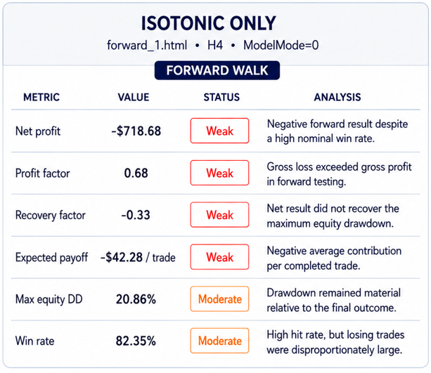
Our first forward walk report uses ModelMode=0 , meaning that the entry probabilities are based on Isotonic Regression without PNN participation. From an initial deposit of USD 10,000, the report registers a net loss of USD -718.68 and a Profit Factor of 0.68. The Recovery Factor is -0.33, while the Sharpe Ratio comes in at -1.33. There were 17 trades, of which 14 were profitable, producing an 82.35% win rate. Maximum equity drawdown reached 20.86%, while maximal balance drawdown was 18.62%.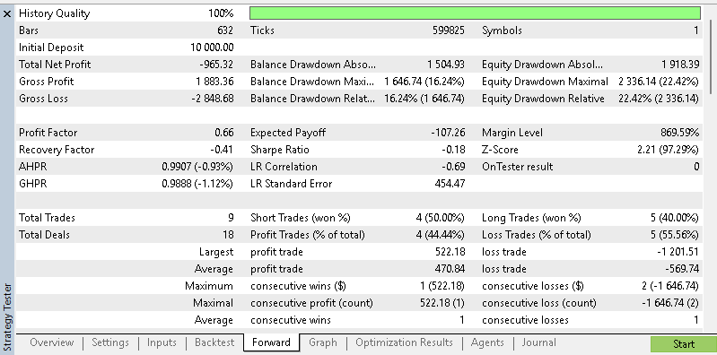

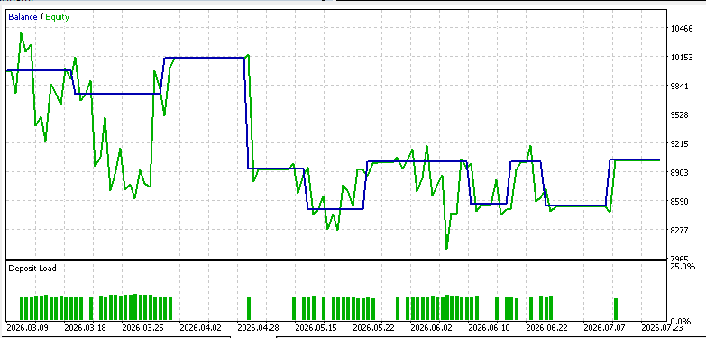
These results therefore give us a more difficult baseline than the earlier example. Despite the high proportion of winning trades, the isotonic-only forward run finished below its starting balance. The explanation is visible in the trade distribution: the largest profitable trade was only USD 125.50, whereas the largest loss reached USD -1,207.37. Average profit was USD 110.10, compared with an average loss of USD -753.34. Thus, a relatively small number of large losses was sufficient to overwhelm a much larger number of winning trades. The isotonic-only model was selective in terms of trade direction, but that selectivity did not translate into positive expectancy during this forward period.

PNN-Enabled Forward Test

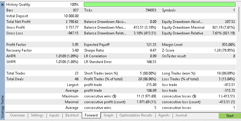
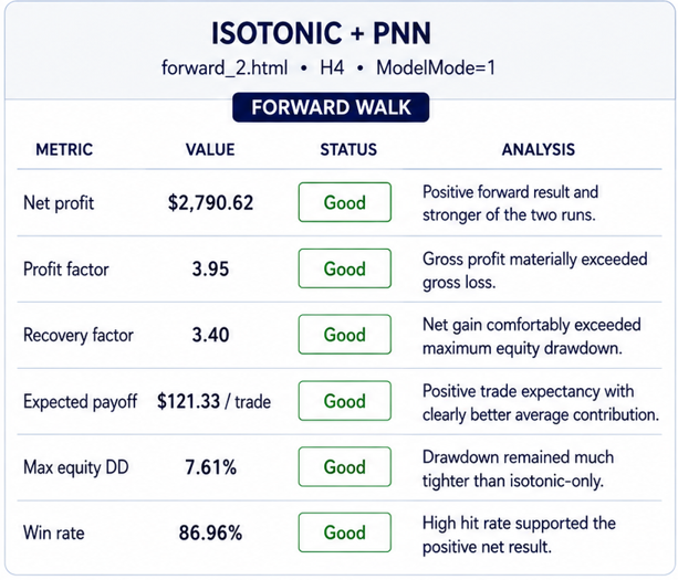
The second report engages ModelMode=1, so Isotonic Regression is supplemented by the PNN. The configuration uses 180 PNN reference samples, with PNNSigma=0.120 and PNNWeight=0.495. The network therefore contributes just under half of the blended probability rather than dominating it. In this run, net profit reaches USD 2,790.62, Profit Factor rises to 3.95, Recovery Factor reaches 3.40, and the Sharpe Ratio comes in at 4.47. The test placed 23 trades, of which 20 were profitable, for an overall win rate of 86.96%. Maximum equity drawdown was 7.61%, while maximal balance drawdown was only 3.18%.

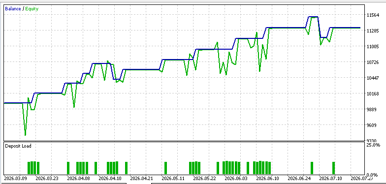
On the face of it, this configuration is considerably stronger. We have positive net profit, a higher Profit Factor, positive risk-adjusted statistics, more trades, and substantially lower drawdown. Average profit was USD 186.89, compared with an average loss of USD -315.72. The largest winner reached USD 215.08, while the largest loss was USD -413.51. The apparent advantage therefore comes not only from maintaining a high win rate, but also from keeping losing trades much smaller relative to those seen in the isotonic-only forward run. This is compatible with the intended filtering role of the PNN, although the result by itself still does not prove that the PNN caused the improvement.

What the Comparison Does Not Isolate

The two reports are still not a clean one-variable ablation. The isotonic-only setup uses an opening threshold of 1, a closing threshold of 4, a price level of -58.0 points, a take-profit level of 26.0 points, and an expiration of 27 bars, equivalent to roughly 108 hours on H4. The PNN-enabled setup instead uses an opening threshold of 3, a closing threshold of 3, a price level of -64.0 points, a take-profit level of 35.5 points, and an expiration of 49 bars, or roughly 196 hours.

There is another complication: the realized forward samples do not begin at the same point. The isotonic-only report begins trading from March 2026, while the PNN-enabled report contains trades from January 2026 onward. The reports therefore differ not only in model configuration and execution settings, but also in the effective forward sample being observed. This makes it too strong to say that adding the PNN alone changed the Profit Factor from 0.68 to 3.95 or transformed a USD -718.68 loss into a USD 2,790.62 profit.

Nonetheless, the reports support a narrower statement: the forward configuration that included the PNN produced the materially stronger result in the supplied tests. One argument in its favor is that PNN filtering may alter signal selectivity enough that different execution settings become appropriate. The counterargument is that those execution differences, together with the different effective forward periods, could explain a meaningful part of the performance gap.

This therefore leaves us with the same need for a follow-up test. A stricter comparison would lock the indicator, calibration, execution, money-management, and forward-period settings so that the only change is ModelMode. Another useful ablation would keep ModelMode=1 but set PNNWeight=0, then progressively restore positive weights. If the improvement reappears consistently as PNN influence is introduced and remains stable across nearby parameter values, the argument for incremental PNN value becomes considerably stronger.

GBPJPY BACKTEST AND FORWARD WALK - PERFORMANCE SUMMARY

January 2025 - August 2026 | Embedded MetaTrader 5 Settings used for Labels

Conclusion

This class turned a regular oscillator problem into a sequence with claims we can test. We implemented seven modes that converted RSI, Stochastic, as well as simple price-context into competing directional hypotheses. Isotonic regression asked the question of if raw ranking deserves an ordered empirical probability. The PNN reopened the compressed score into a six-dimensional state and asked if similar historic neighborhoods were more bullish or bearish. The variables 'RawGate', 'EntryProbability', and 'PNNWeight', helped establish if those views could become an MQL5 trade vote.

Our PNN-enabled forward setps showed higher net profits as well as higher Profit Factor and Sharpe Ratio. We also had more trades and significantly less drawdown when compared to the Isotonic-only setup. Nonetheless the execution settings regarding opening/closing thresholds as well as stop order gaps seemed significant enough that the improved performance cannot be solely attributed to the PNN.

This unresolved attribution helps point to the next testing direction one needs to undertake. Rapid development should not imply finding profitable input settings faster. Arguably, it should instead mean that reaching a comparison capable of rejecting the preferred explanation as quickly as possible. Here, Isotonic-PNN pairing has given us enough evidence to justify a controlled ablation, however not enough to make that ablation unnecessary.

name	description
04.mq5	Wizard assembled Expert Advisor whose header lists referenced code files
SignalIsotonicPNN.mqh	Custom Signal Class file necessary for Wizard Assembly