

A Grid Expert Advisor Based on a Cellular Automaton with Online Learning in MQL5 (Part I): Continuous Adaptation of the Trading Model on Each Bar
 321
 2

Introduction
A trader using a neural network in algorithmic trading for the first time faces a common problem: the network is trained, the backtest looks good, but on a live account, the equity curve begins to decline after three weeks. This is a typical scenario: the model is trained on historical data and has fixed weights that do not account for the new market regime. Periodic retraining helps to some extent, but it requires a pause in trading and supporting infrastructure, and leaves “dead windows” during which no adaptation takes place.
This article is intended for practicing MQL5 Expert Advisor developers and algorithmic traders who need a working out-of-the-box solution, not a theoretical lecture. Specific symptoms of degradation to watch for include a drop in Hit Rate below 50% (with N > 200 predictions), Network Health < 40% (the proportion of profitable cells), a systematic L/S bias > 70/30, and low PrecisionUP/PrecisionDown values for the BPC verifier (50). If these metrics deteriorate, it is not just “noise” from the tester — it is a sign that the fixed weights are becoming outdated.
The solution proposed in this article is not just another MLP with a retraining timer, but an architecture with continuous online adaptation: 10,000 parameters are represented as a cellular automaton (each parameter is an agent), which updates its states on each bar based on a set of features, influences from neighboring cells, and evolution rules; an independent binary predictor operates in parallel (with a 10-bar verification horizon). The article demonstrates which metrics and thresholds to use to assess the system’s “health” and how to diagnose degradation so that corrective action can be taken without stopping trading.
This article systematically examines:
- The problem of fixed weights and degradation criteria
- Online adaptation architecture (CA: cells, features, strategies, rules)
- Independent verification and signal combination (BPC)
- Integration with the grid Expert Advisor and trading parameters
- Practical diagnostics and decision-making thresholds.
Why Fixed Weights Are a Systemic Problem
A classic neural network is trained once using historical data. This is a fundamental limitation: the model describes the market as it was, not as it is. The market changes regimes — from trending to volatile sideways trading, from low to high volatility — while the model continues to search for patterns that no longer exist.
Overfitting to historical data is not a bug, but a direct consequence of the fixed-weight architecture. Any overfitting to past data guarantees a deterioration in performance on live data when the market regime changes.
The standard solution is periodic retraining. The Expert Advisor is stopped, additional data is downloaded, the model is retrained, and the Expert Advisor is restarted. This requires either manual work or complex infrastructure. Most importantly, the model still remains static between retraining sessions.
The solution described in this article is different: the model's parameters are continuously adapted to the market in real time during trading. The tool is a cellular automaton.
What Is a Cellular Automaton, and Why Is It Suitable for This Problem?
A cellular automaton (CA) is a discrete dynamical system. Space is divided into cells, each of which is in a certain state at every moment in time. A cell's next state is determined by its current state and the states of its neighbors, according to a specified rule. Classic examples include Conway's Game of Life and Wolfram's elementary cellular automata.
In the CCellularNeuralNet10K architecture, each cell is a real number in the range [-1, +1], representing the agent’s trading opinion. +1 means “strong long,” -1 means “strong short,” and 0 means neutrality. This value also serves as a dynamic parameter of the model — analogous to a neuron’s weight — but it is updated without interrupting trading.
Key architectural constants:
#define CNN_GRID_W     100   // grid width
#define CNN_GRID_H     100   // grid height
#define CNN_CELLS      10000 // 10 000 parameter cells
#define CNN_FEATURES   50    // entry features
#define CNN_STRATEGIES 10    // archetype strategies
#define CNN_CA_TICKS   6     // automaton steps per forecast
#define CNN_NEIGHBORS  8     // Moore neighbourhood
The 100×100 grid has a toroidal topology: the right edge is connected to the left edge, and the bottom edge is connected to the top edge. The toroidal topology eliminates boundary effects: in a rectangular grid, corner cells have only 3 neighbors instead of 8, creating systemic asymmetry. On a torus, each cell has exactly 8 neighbors.
Neighbor indices are precomputed during initialization and stored in the array `m_nb[CNN_CELLS × 8]`; this is critical for performance. For a single prediction: 10,000 cells × 6 steps × 8 neighbors = 480,000 memory accesses. Precomputation replaces modulo arithmetic with a direct read:
int nx = (x + dx + CNN_GRID_W) % CNN_GRID_W;
int ny = (y + dy + CNN_GRID_H) % CNN_GRID_H;
m_nb[i * CNN_NEIGHBORS + k] = ny * CNN_GRID_W + nx;
50 Market Features: How the Market Is Fed into the Network
The ExtractFeatures() method calculates 50 normalized features from the most recent 200 bars. All features are normalized using MathTanh() to the range [-1, +1] — the same range as the cell states. To speed up the process, cumulative sums of returns and True Range are calculated, which allows any window average to be computed in O(1) time.
| Group | Indices | Description |
|---|---|---|
| Momentum | feat[0..4] | Normalized momentum over 5, 10, 20, 50, and 100 bars |
| Trend Strength | feat[5..9] | DI+/DI− ratio (similar to ADX) over 5, 10, 14, 20, and 50 bars |
| Volatility | feat[10..14] | Normalized ATR over 5, 10, 14, 20, and 50 bars |
| RSI | feat[15..17] | Overbought/Oversold (7, 14, 21) |
| MACD | feat[18..20] | Three settings: (8,17), (12,26), (5,13) |
| Bollinger | feat[21..23] | Price position within the bands (10, 20, 50) |
| Volume | feat[24..26] | Ratio of current tick volume to average tick volume |
| Autocorrelation | feat[27..29] | Serial correlation of returns, lags 1, 2, 5 |
| Mean Reversion | feat[30..32] | Deviation from the 20-, 50-, and 100-period SMAs |
| Price Level | feat[33..35] | Price position within the ranges over the last 20, 50, and 100 bars |
| Hurst | feat[36..37] | Hurst exponent over 30 and 100 bars |
| Candlestick Analysis | feat[38..41] | Candlestick body/shadows, opening gap |
| Acceleration | feat[42..44] | Momentum derivative, change in volatility |
| interaction features | feat[45..47] | Momentum × Volume, Trend/Volatility, RSI × Bollinger Bands |
| Time | feat[48..49] | sin and cos of the hour (cyclic encoding) |
The Hurst exponent (feat[36..37]) describes the long-term memory of a time series: H > 0.5 corresponds to a trending market, H < 0.5 to a mean-reverting market, and H ≈ 0.5 to a random walk. The calculation is performed using rescaled range analysis (R/S analysis):
double hurst = MathLog(range_rs / std_rs) / MathLog((double)w); // Normalization: +1 = trend, -1 = mean reversion
feat[36 + p] = (hurst - 0.5) * 2.0;
If feat[36] is close to +1, the cells' trend-based strategies are boosted by rule R12. If it is close to -1, mean-reversion strategies take the lead. The system switches between modes automatically.
Cyclical time encoding (feat[48..49]) — sine and cosine of the hour:
double hour_norm = dt.hour / 24.0 * 2.0 * M_PI;
feat[48] = MathSin(hour_norm);
feat[49] = MathCos(hour_norm);
Sine and cosine ensure that 23:00 and 01:00 are “close” in feature space (distance ≈ 0.26), even though the numbers 23 and 1 are far apart. Linear encoding of the hour would create an artificial discontinuity at midnight.
10 Archetypal Strategies: Cell Genes
Each cell is assigned to one of 10 strategies — this is its “gene.” Upon initialization, the distribution is uniform: 1,000 cells per strategy. Initialization ensures complete coverage of the feature space:
m_strategy[i] = i % CNN_STRATEGIES;
m_feat_idx[i] = (i / CNN_STRATEGIES) % CNN_FEATURES; // 10 × 50 = 500 pairs, with 20 cells in each
A strategy's signal is a weighted combination of features specific to its market hypothesis:
case CNN_TREND_SHORT:
   //--- Short-term trend: momentum + trend strength + volatility
   return 0.5 * feat[0] + 0.3 * feat[5] + 0.2 * feat[10];

case CNN_REVERSAL:
   //--- Reversal: RSI + Bollinger Bands + mean reversion
   return -0.4 * feat[16] - 0.4 * feat[22] + 0.2 * feat[30];

case CNN_MEAN_REV:
   //--- Mean reversion: SMA50 + RSI14 + Hurst exponent
   return -0.5 * feat[31] - 0.3 * feat[17] + 0.2 * feat[37];

case CNN_CONSENSUS:
   //--- Consensus: 70% neighbor average + 30% own signal
   return nb_mean * 0.7 + feat[0] * 0.3;
The CNN_CONSENSUS strategy is a special case: these cells vote in concert with their neighbors. They reinforce the consensus, but they do not create it. This is the network's built-in inertia.
Important: A strategy is not a permanent attribute of a cell. Under rule R7, a cell changes its strategy after three consecutive loss-making predictions. The distribution of strategies across the network continuously adapts to the current market regime.
12 Rules of Cell Evolution
In each of the 6 CA steps, each cell computes a new state. Base signal — 50% from the primary feature, 30% from the strategy, 20% from the neighbors' average:
double primary   = feat[m_feat_idx[i]] * 0.5;
double strat_sig = GetStrategySignal(m_strategy[i], feat, nb_mean) * 0.3;
double nb_signal = nb_mean * 0.2;
double new_state = primary + strat_sig + nb_signal;
Next, evolution rules are applied to modify the base signal. Below are the key ones.
R1–R2: PnL as a signal amplifier. Profitable cells “speak louder” — analogous to an attention mechanism:
if(pnl_i > 0)
   new_state *= 1.0 + 0.2 * MathMin(pnl_i, 1.0);
else
   new_state *= MathMax(0.4, 1.0 + 0.3 * pnl_i);
R3: Social consensus among neighbors. If 5 out of 8 neighbors agree, the cell gently aligns with the majority:
if(nb_agree >= 5.0 / 8.0)
  {
   new_state = new_state * (1.0 - nb_agree * 0.4) +
               msign * MathAbs(new_state) * nb_agree * 0.4;
  }
R5: High volatility reduces confidence. In a chaotic market, signals are dampened — the Expert Advisor does not enter trades under uncertainty:
if(feat[12] > 0.3)
   new_state *= MathMax(0.4, 1.0 - feat[12] * 0.4);
R6: A confirmed trend is reinforced. When the short-term and medium-term trends align, the cells receive additional momentum:
if(feat[7] * feat[2] > 0.05)
  {
   double boost = MathMin(0.3, MathAbs(feat[7]) * 0.4);
   new_state += sign(feat[7]) * boost;
  }
R7: Switching strategies after a series of losses. Three consecutive losses — the cell switches to the adjacent strategy:
if(m_losses[i] >= 3)
  {
   m_strategy[i] = (m_strategy[i] + 1 + MathRand() % 3) % CNN_STRATEGIES;
   m_losses[i] = 0;
  }
R8: Global consensus drives the network toward consensus. When 70% or more of the cells agree in the same direction, the network begins to reinforce this consensus:
if(MathAbs(consensus) > 0.7)
  {
   double csign = (consensus > 0) ? 1.0 : -1.0;
   new_state = 0.6 * new_state + 0.4 * csign * MathAbs(new_state);
  }
R12: Fractal inertia in a trending market. In a trending market, the cell “remembers” its previous opinion:
if(feat[36] > 0.2)
   new_state = 0.7 * new_state + 0.3 * m_state[i]; // 30% weight assigned to the previous state
Together with OptimizeParameters(), which reassigns weak cells (capital < 0.15) to random strategies, this allows the network to continuously explore the space of possibilities without getting stuck in local minima.
Weighted Voting and Automatic Bias Correction
After 6 CA steps, the final forecast is a weighted average of the forecasts from 10,000 cells. A cell's weight depends on its accumulated authority:
double WeightedVote()
  {
   double wsum = 0.0, wtotal = 0.0;

   for(int i = 0; i < CNN_CELLS; i++)
     {
      double w = m_capital[i] * (1.0 + MathMax(0.0, m_pnl[i]) * 0.005);
      wsum   += m_state[i] * w;
      wtotal += w;
     }

   double vote = wsum / wtotal + m_bias;
   return MathTanh(vote * 2.0);
  }
Cells whose capital approaches 0.05 (the lower bound) have almost no influence on the final result. Cells with high accumulated PnL have a weight that is proportionally greater than the base weight.
Automatic correction of systematic bias is triggered when there is an imbalance between long and short predictions over the last 200 or more forecasts:
if(total_sig > 200)
   m_bias = 0.15 * (double)(m_short_cnt - m_long_cnt) / total_sig;
This is a safeguard against systematic bias that arises in trending markets where one direction predominates.
Binary Predictor: A Second Independent Horizon
CBinaryPredictor10K addresses a problem that is fundamentally different from that of the main CA: not “where the market is heading right now,” but “will the price be higher or lower in 10 bars?” This is the prediction horizon of the grid Expert Advisor. If BPC predicts that the price will be higher in 10 bars, opening a BUY grid makes more sense than relying solely on the current momentum.
The key mechanism is a ring buffer for forecast verification. On each bar, OnNewBar() performs two actions simultaneously:
//--- Verification of the forecast made BPC_HORIZON bars ago
int    verify_idx = m_ring_idx;
double curPrice   = r[0].close;
double predPrice  = m_ring[verify_idx].price;

//--- Recording of a new forecast in the same ring buffer slot
m_ring[m_ring_idx] = {direction=dir, price=curClose, confidence=conf, valid=true};
m_ring_idx = (m_ring_idx + 1) % BPC_HORIZON; // A single index handles both verification of the past forecast and recording of the new forecast
BPC maintains a complete confusion matrix with accuracy broken down by direction:
double GetPrecisionUp()
  {
   int tp_fp = m_true_pos + m_false_pos;
   return (tp_fp > 0) ? (double)m_true_pos / tp_fp : 0;
  }
double GetPrecisionDown()
  {
   int tn_fn = m_true_neg + m_false_neg;
   return (tn_fn > 0) ? (double)m_true_neg / tn_fn : 0;
  }
If PrecisionUP = 65% and PrecisionDown = 48%, the system is statistically significant only for long positions. The Expert Advisor takes this into account when combining signals.
Combining Signals from Two Engines
On each new bar, the Expert Advisor combines CA and BPC signals:
double vote   = g_ca.PredictNextMove(_Symbol); // current momentum
int    bpcDir = g_bpc.GetLastDirection();      // BPC direction
double bpcAcc = g_bpc.GetAccuracy();

//--- Combining Signals from Two Independent Engines
if(bpcAcc > 0.55)
  {
   int caDir = (vote > 0) ? 1 : -1;

   if(bpcDir == caDir)
      effConf *= 1.0 + (bpcAcc - 0.5) * 2.0;               // increased confidence when signals agree
   else
      effConf *= MathMax(0.3, 1.0 - (bpcAcc - 0.5) * 2.0); // decreased confidence when signals conflict
  }
Two independent engines with different prediction horizons vote on the direction. Agreement boosts confidence; disagreement undermines it. This is built-in real-time cross-validation.
Three-Level Online Learning
The system learns across three time horizons simultaneously.
On each bar. After each new bar, the previous CA forecast is compared with the actual price movement. The PnL and authority of all 10,000 cells are updated:
void UpdateStats(int hour, bool correct, double prediction, double actual_move)
  {
   for(int i = 0; i < CNN_CELLS; i++)
      UpdateCellPnL(i, m_state[i], actual_move); // updating the cell's performance based on actual price movement
  }
After closing the grid. The actual financial result is passed on — cells that voted for the profitable direction gain authority:
//--- Genome's response to a loss-making trade cycle
if(avgProfit < 0)
  {
   g_genome[s].sl_factor   *= 1.05;
   g_genome[s].risk_factor *= 0.92;
   g_genome[s].grid_step   *= 1.05;
  }

//--- Genome's response to a series of inconsistent results
if(stability < 0.3)
  {
   g_genome[s].risk_factor *= 0.88;
   g_genome[s].lot_mult    *= 0.97;
   g_genome[s].max_levels  -= 1;
  }
Every 15 forecasts. Cells with capital < 0.15 are restructured: they are assigned a random strategy and feature, and their capital is restored to 0.25. This is evolutionary selection — weak configurations are displaced by mutations.
Evolution of the Expert Advisor's Parameters
The Expert Advisor supports five trading-parameter genomes — ranging from aggressive to conservative. Every 5 trading cycles, the genomes mutate based on past performance:
//--- Parameter mutation following a loss-making trading cycle
if(avgProfit < 0)
  {
   g_genome[s].sl_factor   *= 1.05;
   g_genome[s].risk_factor *= 0.92;
   g_genome[s].grid_step   *= 1.05;
  }

//--- Reducing aggressiveness during a streak of inconsistent results
if(stability < 0.3)
  {
   g_genome[s].risk_factor *= 0.88;
   g_genome[s].lot_mult    *= 0.97;
   g_genome[s].max_levels  -= 1;
  }
All of the Expert Advisor's parameters are calculated using ATR and genomes. The only input parameter is the Magic Number.
Integration with a Simple and Lightweight Grid Expert Advisor
The ComputeGridParams() method translates the CA vote into specific trading instructions:
struct CAGridDecision
  {
   double raw_vote;       // raw forecast [-1..+1]
   int    direction;      // +1 long, -1 short, 0 neutral
   double confidence;     // confidence = |vote|
   int    grid_step;      // dynamic grid step in points
   double lot_multiplier; // lot-size multiplier
   bool   reverse_signal; // a reversal signal for the entire grid
   bool   close_signal;   // forced closure signal
   string reason;         // text log for diagnostics
  };
The dynamic grid step scales based on volatility. In a calm market, the step size shrinks to 0.5× the base value; in a volatile market, it expands to 3×:
//--- Scaling the grid step based on current volatility
stepScale = 1.0 + (feat[12] + 1.0) * 0.5;

//--- Limiting the grid step size to a safe range
stepScale = MathMax(0.5, MathMin(3.0, stepScale));
decision.grid_step = (int)MathRound(baseGridStep * stepScale);
A reversal signal is triggered if a position contradicts a confident CA forecast (confidence ≥ 0.25):
if((isLong && caShort) || (!isLong && caLong))
   decision.reverse_signal = true;
A closing signal is triggered at a deep grid level when confidence is lost — the network acknowledges its mistake before the final level is reached:
if(currentLevel >= maxLevels / 2 && decision.confidence < 0.03)
   decision.close_signal = true;
Expert Advisor Skeleton
#include <Cellular10K\CellularNeuralNet10K.mqh>
#include <Cellular10K\CellularBinaryPredictor10K.mqh>

input int InpMagicNumber = 777777; // the Expert Advisor's only input parameter

CCellularNeuralNet10K *g_ca  = NULL;
CBinaryPredictor10K   *g_bpc = NULL;

int OnInit()
  {
   g_ca  = new CCellularNeuralNet10K();
   g_bpc = new CBinaryPredictor10K();

   g_ca.Initialize();
   g_bpc.Initialize();

   CalibrateGenomes();
   return INIT_SUCCEEDED;
  }

void OnTick()
  {
   SyncGridState();
   TrackDrawdown();
   CheckStopLoss();

   //--- Managing an Already Open Grid
   if(g_direction != 0)
     {
      CheckTakeProfit();
      CheckMaxHold();
      ManageGrid();
     }

   if(IsNewBar())
      HandleNewBar();

   ShowStatus();
  }

void HandleNewBar()
  {
   VerifyPrediction();

   //--- Verifying the previous BPC forecast and recording the new forecast
   g_bpc.OnNewBar(_Symbol);

   //--- Recalculation of the active genome based on the history of trading cycles
   ComputeOptimalParams();

   double vote    = g_ca.PredictNextMove(_Symbol);
   double effConf = CombineSignals(vote, g_bpc);

   //--- Checking the conditions for a new entry
   if(g_direction != 0)
      return;
   if(effConf < g_cur.min_conf)
      return;

   int dir = (vote > 0) ? 1 : -1;
   OpenPosition(dir, 0);
  }
Network Health Metrics
What to Watch
PrintDetailedStats() writes the network status to the log. An example of actual output after more than 4,800 predictions:
| Metric | Value |
|---|---|
| Total Predictions | 4821 |
| Hit Rate | 58.34% |
| Best Hit Rate | 63.12% |
| Network Health | 67.3% (6,730 out of 10,000 cells are profitable) |
| Top Cell #1 | Cell[23,45] TREND_M F:7 Cap:0.987 PnL:0.00412 |
| Top Cell #2 | Cell[71,12] MOMENTUM F:1 Cap:0.972 PnL:0.00389 |
| TREND_S | 1,023 cells, PnL: +0.4821 |
| REVERSAL | 987 cells, PnL: −0.1203 |
| BPC 10bar UP | Accuracy: 61.2% (47 verifications), P+63%, P−59% |
| Metric | Normal | Alarm | Interpretation |
|---|---|---|---|
| Network Health | > 60% | < 40% | Percentage of profitable cells. < 40% — the market has invalidated the current configuration |
| Hit Rate (>200 predictions) | > 55% | < 50% | A significant edge is present. < 50% — check the direction logic |
| CONSENSUS Share | < 20% | > 20% | The network has "given up" and is repeating itself |
| BPC Precision+ / Precision- | > 58% | < 52% | Statistically significant with more than 50 verifications (N > 50) |
| Signal Balance L/S | 40/60–60/40 | > 70/30 | Systematic bias; bias correction helps to some extent |
Network Health is the primary indicator of adaptation. A gradual decline from 67% to 50% is normal during a market regime shift; automatic restructuring should restore the value within 50–100 bars. A sharp drop below 40% over 10–15 bars is a sign of abnormal market movement (a news shock or gap).
After adaptation, Strategy Distribution shows which market regime is dominant. In a trending market, the share of TREND_S/TREND_M/TREND_L increases, while the shares of REVERSAL and MEAN_REV decrease. This is normal and to be expected — that is exactly why Rule R7 exists.
Comparison with Fixed Architectures
The figures shown are approximate values observed during a test run on EURUSD H1. Specific results depend on the time period, the instrument, and the market regime.
| Architecture | Hit Rate (EURUSD H1) | Adaptation to Market Regime Changes |
|---|---|---|
| Fixed-Weight MLP | ~51% | No (requires retraining) |
| MLP with weekly retraining | ~53% | Partial |
| BPC only (10-bar prediction horizon) | ~54% | Partial |
| CA 10K without BPC | ~56% | Continuous |
| CA 10K + BPC (full architecture) | ~58% | Continuous + cross-verification |
The key difference lies not in absolute accuracy, but in how the system behaves when the market regime changes. An MLP with fixed weights degrades gradually and imperceptibly. The inner workings of the CA architecture are visible: Network Health and Strategy Distribution show adaptation in real time.
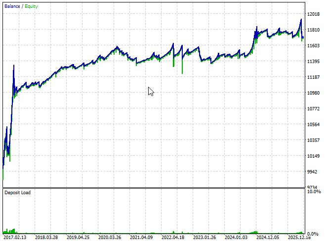
A backtest of the system covering the 2017–2026 period, using OHLC simulation on the H1 timeframe (EUR/USD), demonstrates the system’s stability, though the results are not perfect:
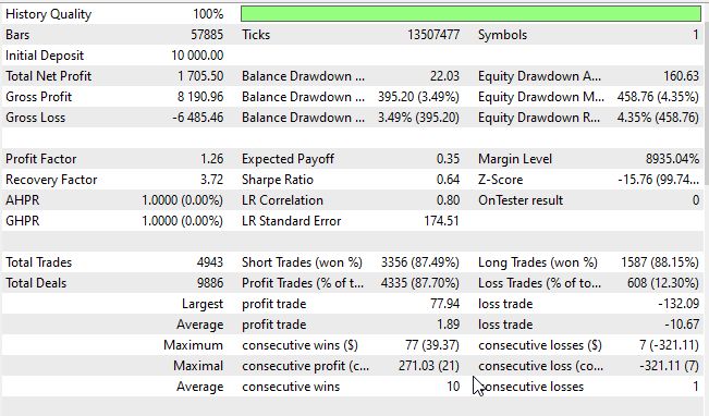
The metrics — the Sharpe ratio and profit factor — are also rather weak:
What the Trader Gets
A trader ran into a problem: a neural network with fixed weights degrades in the live market after a few weeks. The solution lies not in more frequent retraining or a deeper network, but in a different way of conceptualizing a parameter. In this architecture, each of the 10,000 parameters is an agent that competes, evolves, and is deactivated during trading. The binary predictor independently verifies forecasts every 10 bars. The five trading-parameter genomes change (mutate) based on cycle history.
Three MQL5 files, zero external dependencies, one input parameter.
Success criteria and practical steps for getting started:
- Recommended starting setup: EURUSD H1, default Magic Number.
- Monitoring during the first 200–300 predictions: Hit Rate should approach >55% (statistically significant at N>200), while Network Health ≳ 60% is considered normal; BPC PrecisionUP/PrecisionDown >58% at N>50 is statistically significant. If, after 300 predictions, Hit Rate is ≤ 52%, check Network Health, the L/S balance, and min_conf in the logs.
- Caution: If the CONSENSUS share is >20% or L/S is >70/30, this indicates a systematic bias; run diagnostics and analyze dominant strategies and feature distribution.
Now, instead of infrequent “retraining” and inactive weights, the system updates its parameters on every bar (rules R1–R12 respond to PnL, volatility, the Hurst exponent, and agreement among neighboring cells), weak cells are replaced, trading-parameter genomes mutate, and BPC limits false entries over the prediction horizon. This eliminates "dead windows" and provides measurable adaptation metrics (Network Health, Strategy Distribution, BPC precision) that can be used to determine whether the underlying degradation issue has been resolved.
A brief checklist of steps to take if performance metrics deteriorate:
- If Hit Rate drops and Network Health is <40%, allow 50–100 bars for restructuring; if that does not help, reduce min_conf and/or analyze the strategy distribution.
- If BPC loses accuracy, check the number of verifications (N), recalibrate, or temporarily reduce BPC's influence when combining signals.
- Strong L/S bias: enable bias correction and analyze the cause (a news shock, a change in volatility, or feature failures).
The result is a practical implementation of the idea: a shift from “fixed weights” to online parameter evolution with clear health metrics and diagnostic tools — without the need to pause trading for retraining.
| File name | File description |
|---|---|
| CA_Grid_10K.mq5 | The system's main grid Expert Advisor |
| CellularNeuralNet10K.mqh | Include file for trading cellular automata; place it in Include\Cellular10K |
| CellularBinaryPredictor10K.mqh | Include file for predictive cellular automata; place it in Include\Cellular10K |
Translated from Russian by MetaQuotes Ltd.
Original article: https://www.mql5.com/ru/articles/22211
Warning: All rights to these materials are reserved by MetaQuotes Ltd. Copying or reprinting of these materials in whole or in part is prohibited.
This article was written by a user of the site and reflects their personal views. MetaQuotes Ltd is not responsible for the accuracy of the information presented, nor for any consequences resulting from the use of the solutions, strategies or recommendations described.



 Features of Custom Indicators Creation
 From Basic to Intermediate: Technical Indicators (II)
 Features of Experts Advisors
 Building a Trade Replay Tool in MQL5

- Free trading apps
- Over 8,000 signals for copying
- Economic news for exploring financial markets
You agree to website policy and terms of use