Using Renko-bar Regression with Error Correction

In the previous article, we discussed a classification-based approach to forecasting Renko bars using CatBoost: the model predicted the direction of the next bar (up or down) and achieved an accuracy of about 59%. In this article, we will take the next step and move from classification to regression: we will predict not only the direction but also the magnitude of the logarithmic return of the next Renko bar. This provides additional information for making trading decisions — we get not just a binary signal, but a numerical forecast of price movement with a confidence interval.

The main problem with any regression model based on financial data is systematic error, or forecast bias. A model trained on historical data may systematically overestimate movements in one direction and underestimate them in the other. We will show how to identify and correct this error using a two-step scheme. First, a multi-stage cascade of residual models is used, where each subsequent model learns from the errors of the previous one. Then a final conditional bias correction is performed. The result will be a production trading system that works with real daily EURUSD data from MetaTrader 5 and generates a trading signal with the calculated position size, stop-loss, and take-profit in units of the Renko brick size.

Renko charts have an important property: the size of each bar is fixed and equal to brick_size. This means that when forecasting the next bar, the target is effectively discrete. It takes three values: +log(1 + brick_size/close) when moving up by one brick; -log(1 - brick_size/close) when moving down; and a rare zero value at reversal points, when the close of the current bar coincides with the boundary. It would seem that this is an ideal task for classification.

However, regression on such a target offers two advantages that are important to understand from the very beginning. The model returns not just a class, but a continuous value that can be interpreted as confidence in the forecast. A forecast of +0.0042 means “almost certainly up by one brick,” while a forecast of +0.0005 means “technically up, but the model is not sure.” This gradation is useful for filtering out weak signals. In addition, the regression formulation naturally extends to horizons of more than one bar: if you set `horizon=3` or `horizon=5` instead of `horizon=1`, the target becomes continuous, and the model begins to estimate not only the direction but also the strength of the trend. In this article, we consider `horizon=1` and predict the next brick. This is the cleanest formulation of the problem, and it is a convenient way to demonstrate the error correction mechanism.

Brick Size and the Construction of Renko Bars

The brick size determines the resolution of the Renko chart. If the `brick_size` is too small, the chart gets swamped with noise; if it is too large, we miss significant moves. We use the classic approach: `brick_size` is calculated as ATR(14) multiplied by a factor of 0.5.

def _calc_atr(df: pd.DataFrame, period: int = 14) -> pd.Series:
    tr = pd.concat([
        df["high"] - df["low"],
        (df["high"] - df["close"].shift()).abs(),
        (df["low"] - df["close"].shift()).abs(),
    ], axis=1).max(axis=1)
    return tr.rolling(period).mean()


def create_renko_bars(df, brick_size=None, atr_multiplier=0.5):
    if brick_size is None:
        atr = _calc_atr(df, 14)
        brick_size = float(atr.mean() * atr_multiplier)
    # ... bar construction

For daily EURUSD over the 2024–2025 period, the `brick_size` comes out to about 0.004 — roughly 40 pips. This is a reasonable size for a daily strategy: the Renko chart smooths out intraday noise and preserves structural movements. An important aspect of implementation is handling reversals. In classic Renko, for a trend reversal to occur, the price must move a distance of 2×brick_size from the extreme, not just one brick. This is modeled by adding an extra brick when the direction changes, using the simple condition `if current_direction is not None and direction != current_direction: num_bricks += 1`.

Features

For each data point, we generate 25 features that describe the context of the last 10 Renko bars. The features cover the historical sequence of movements (directions `dir_0` ... `dir_9`), aggregates by direction (the share of upward bars, streak lengths, and the number of direction changes), volume characteristics (latest and average volume, their ratio, and the linear volume trend over the window), and price structure (range, average move size, and latest and cumulative returns).

feat = {
    **{f"dir_{j}": int(w_dirs[-(j + 1)]) for j in range(lookback)},
    "up_ratio": float((w_dirs > 0).mean()),
    "last_dir": int(w_dirs[-1]),
    "dir_changes": int(np.sum(np.abs(np.diff(w_dirs)) > 0)),
    "last_up_streak": int(up_streaks[i - 1]),
    "last_down_streak": int(dn_streaks[i - 1]),
    "max_up_streak": int(up_streaks[i - lookback:i].max()),
    "max_down_streak": int(dn_streaks[i - lookback:i].max()),
    "last_volume": float(w_vols[-1]),
    "avg_volume": float(avg_vol),
    "volume_ratio": float(w_vols[-1] / avg_vol),
    "volume_trend": float(np.polyfit(range(lookback), w_vols, 1)[0]),
    "price_range": float(w_closes.max() - w_closes.min()),
    "range_per_bar": float(brick_proxy),
    "last_return": float(np.log(w_closes[-1] / w_closes[-2])),
    "cum_return": float(np.log(w_closes[-1] / w_closes[0])),
}

The regression target is the logarithmic return over a horizon of `horizon` Renko bars, calculated as `target = float(np.log(closes[i - 1 + horizon] / closes[i - 1]))`. The logarithmic form is preferable to a simple price difference: it is symmetric with respect to sign, scale-invariant, and naturally additive when aggregating forecasts across different horizons.

Cascade of Residual Models

The classic cascade architecture looks like this. We train the first model, M₀, on the original data (X, y). This model outputs a prediction ŷ₀ = M₀(X) and leaves residuals r₀ = y - ŷ₀. Next, we train a second model, M₁, on the same features X, but this time we predict the residuals r₀ rather than the original y. The forecast is updated as follows: ŷ₁ = ŷ₀ + η × M₁(X), where η is the shrinkage coefficient, which is less than 1 (in our case, η = 0.6). The new residuals, r₁ = y - ŷ₁, are used to train the next model, M₂, and so on. The final raw cascade forecast is expressed as ŷ = M₀(X) + η×M₁(X) + η×M₂(X) + ... + η×Mₖ(X).

Why is this not the same as simply increasing the number of iterations in a single CatBoost model? There are three fundamental differences.

Each residual model has its own early stopping mechanism. The base model stops training when the validation metric on the target y stops improving. Residual models stop on residual targets, which have a different structure: they are noisier and less predictable.

Between cascade stages, the residuals are recalculated using OOF predictions obtained with TimeSeriesSplit, which ensures there is no future leakage: the residual model learns to predict residuals that the base model did not see during training. Without this mechanism, the cascade would overfit instantly.

A separate early stopping mechanism operates at the cascade level. If the next stage does not improve the OOF-MAE by more than min_improvement, the stage is rejected. After several consecutive rejected stages, the cascade stops.

The main training loop is shown below:

# Stage 0 — Base Model
oof_cum, base_model = self._compute_oof(X, y, stage_idx=0)
mae_stage = mean_absolute_error(y[valid], oof_cum[valid])
self.stages.append(CascadeStage(model=base_model, oof_mae=mae_stage, shrinkage_applied=1.0))

best_mae = mae_stage
no_improve_count = 0

# Iterative residual stages
for s in range(1, self.max_stages + 1):
    residuals = y - oof_cum
    X_s = X.loc[valid].reset_index(drop=True)
    r_s = residuals[valid]
    
    oof_r, stage_model = self._compute_oof(X_s, r_s, stage_idx=s)
    oof_cum_updated = oof_cum.copy()
    oof_cum_updated[idx_valid[mask_inner]] = (
        oof_cum[idx_valid[mask_inner]] + self.shrinkage * oof_r[mask_inner]
    )
    
    mae_new = mean_absolute_error(y[valid_new], oof_cum_updated[valid_new])
    improvement = best_mae - mae_new
    
    if improvement > self.min_improvement:
        self.stages.append(CascadeStage(
            model=stage_model, oof_mae=mae_new, shrinkage_applied=self.shrinkage
        ))
        oof_cum = oof_cum_updated
        best_mae = mae_new
        no_improve_count = 0
    else:
        no_improve_count += 1
        if no_improve_count >= self.patience:
            break

CatBoost parameters differ between the base and residual stages. The base model uses 500 iterations, learning_rate=0.03, depth=6, and L2 regularization with a value of 3.0. The residual models are smaller and more strongly regularized: 300 iterations, learning_rate=0.02, depth=4, L2=5.0. The reason is simple: the residuals consist of noise plus a small residual structure, and deep trees trained on such data will quickly start capturing noise instead of signal, which is why stronger regularization is critical for convergence.

def _base_params(self, stage_idx):
    is_base = (stage_idx == 0)
    return {
        "iterations": 500 if is_base else 300,
        "learning_rate": 0.03 if is_base else 0.02,
        "depth": 6 if is_base else 4,
        "loss_function": "RMSE",
        "l2_leaf_reg": 3.0 if is_base else 5.0,
        "random_seed": 42 + stage_idx,
        "early_stopping_rounds": 40,
    }

Conditional Bias Correction

Even after the cascade, a systematic error may still remain in the OOF predictions. For example, the model may, on average, overestimate bullish predictions (when `raw_pred` is greater than zero) and underestimate bearish ones. We detect and compensate for this using conditional bias correction. The algorithm is simple: on the OOF predictions, we calculate the residuals as `residuals = y_pred - y_true`. A positive average residual means that the model is overestimating, so this bias must be subtracted from the prediction. We calculate the bias separately for positive predictions (`bull_bias`) and negative predictions (`bear_bias`).

@dataclass
class BiasCorrector:
    def fit(self, y_true, y_pred_oof):
        residuals = y_pred_oof - y_true
        self.global_bias = float(np.mean(residuals))
        self.residual_std = float(np.std(residuals, ddof=1))
        
        if self.method == "conditional":
            bull = y_pred_oof > 0
            bear = y_pred_oof < 0
            self.bull_bias = float(np.mean(residuals[bull])) if bull.sum() > 5 else self.global_bias
            self.bear_bias = float(np.mean(residuals[bear])) if bear.sum() > 5 else self.global_bias
        return self
    
    def correct(self, raw_pred):
        if self.method == "conditional":
            if raw_pred > 0:
                return raw_pred - self.bull_bias
            if raw_pred < 0:
                return raw_pred - self.bear_bias
        return raw_pred - self.global_bias

An important safeguard against degradation is the guard. If conditional bias correction worsens the OOF-MAE (sometimes the data is already nearly symmetric, and the correction merely adds noise), it is automatically disabled: all biases are set to zero, and the final prediction equals the cascade’s raw prediction. The `residual_std` parameter is used to construct a 95% confidence interval for the final prediction using the standard formula `pred ± 1.96 × residual_std`.

Production Trading System on MetaTrader 5

Everything we have built is assembled into a single production script: `RenkoBattle_EURUSD_D1.py`. It connects to MetaTrader 5, loads data, trains or loads a saved model, generates a trading signal, and — with explicit permission — submits an order. Connection to the terminal and data loading are implemented via the standard MetaTrader5 API::

def mt5_connect(cfg):
    if not mt5.initialize(path=cfg.get("mt5_terminal_path")):
        return False
    info = mt5.account_info()
    print(f"[MT5] Account: {info.login} @ {info.server}, balance={info.balance:.2f}")
    return True


def mt5_fetch_ohlc(symbol, timeframe, days):
    mt5.symbol_select(symbol, True)
    end = datetime.now()
    start = end - timedelta(days=days)
    rates = mt5.copy_rates_range(symbol, timeframe, start, end)
    df = pd.DataFrame(rates)
    df["time"] = pd.to_datetime(df["time"], unit="s")
    return df

If the saved model becomes outdated (the market regime has changed, or ATR has shifted significantly), the script automatically retrains it. The ratio of the new `brick_size` to the one that was in the model at the time of training is checked at every run: if this ratio falls outside the range of 0.7–1.4, a full retraining cycle is initiated and the saved model is overwritten.

The model's forecast is converted into a specific order with SL and TP expressed in `brick_size` units. The spread filter rejects signals whose expected price movement does not exceed the current spread by more than 1.5 times — this protects against entries in noisy market conditions. The stop-loss is set at a distance of two bricks, and the take-profit at three bricks, resulting in a risk-to-reward ratio of 1:1.5. The position size is calculated based on a fixed risk of 0.5% of the balance. The SL size in points is multiplied by the point value for 1 lot — this gives us the loss per 1 lot. The monetary risk is then divided by this loss to arrive at the required volume. The volume is then rounded to the broker's volume step and limited to the minimum and maximum permissible values.

def build_signal(prediction, symbol, brick_size, cfg):
    info = mt5.symbol_info(symbol)
    tick = mt5.symbol_info_tick(symbol)
    
    # Spread Filter
    expected_move_abs = abs(prediction["expected_move_pct"]) / 100.0
    spread_frac = info.spread * info.point / prediction["last_close"]
    if expected_move_abs < spread_frac * 1.5:
        return {"action": "NONE", "reason": "signal_below_spread"}
    
    sl_distance = cfg["sl_in_bricks"] * brick_size
    tp_distance = cfg["tp_in_bricks"] * brick_size
    
    if prediction["direction"] == "UP":
        entry = tick.ask
        sl = entry - sl_distance
        tp = entry + tp_distance
        order_type = mt5.ORDER_TYPE_BUY
    else:
        entry = tick.bid
        sl = entry + sl_distance
        tp = entry - tp_distance
        order_type = mt5.ORDER_TYPE_SELL
    
    # Risk-Based Position Sizing
    account = mt5.account_info()
    risk_amount = account.balance * cfg["risk_per_trade_pct"] / 100.0
    sl_points = sl_distance / info.trade_tick_size
    loss_per_lot = sl_points * info.trade_tick_value
    raw_volume = risk_amount / loss_per_lot
    volume = max(info.volume_min, 
                 min(info.volume_max, 
                     round(raw_volume / info.volume_step) * info.volume_step))
    
    return {
        "action": "BUY" if prediction["direction"] == "UP" else "SELL",
        "order_type": order_type,
        "entry_price": entry, "sl": sl, "tp": tp,
        "volume": volume, "risk_amount": risk_amount,
    }

The script implements a three-level safeguard against accidentally launching live trading. In the default configuration, `enable_trading=False` and `dry_run=True` are set, and the explicit CLI flag `--trade` is required. When the system is launched with the command `python RenkoBattle_EURUSD_D1.py`, it only displays a report with the forecast and model metrics, without sending anything to the broker. The command `python RenkoBattle_EURUSD_D1.py --retrain` forces the model to be retrained, while live trading is enabled only by the explicit command `python RenkoBattle_EURUSD_D1.py --trade`. This allows you to safely test the system in watch-only mode for an unlimited amount of time and begin trading only after its behavior has been fully verified.

Results for Daily EURUSD

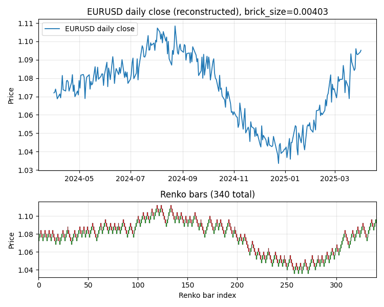
We applied the complete system to EURUSD D1 data for the period from April 2024 to April 2025 (approximately 270 trading days). Parameters: lookback=8, horizon=1, atr_multiplier=0.5, max_stages=12, patience=3, shrinkage=0.6. After loading the D1 data and constructing a Renko chart with an adaptive `brick_size`, we obtained 340 Renko bars from 273 trading days. It is clear that the Renko representation smooths out daily fluctuations and clearly highlights structural movements: an upward phase in the summer of 2024, a correction in the autumn, a drop in winter to 1.04, and a recovery in spring 2025.

The cascade accepted only one residual stage. The base model yielded an OOF MAE of 0.001306; after the first residual stage, the MAE decreased to 0.001287 (an improvement of 1.9e-5). The next three stages were rejected — their contribution was less than min_improvement or even negative. Early stopping was triggered correctly after three consecutive rejected stages.

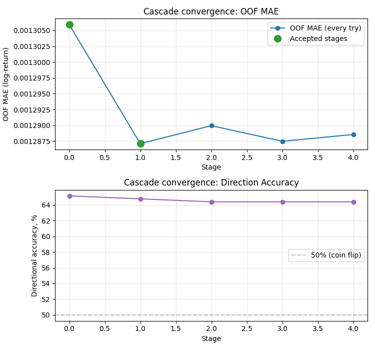
Direction accuracy remains at 64.4% — consistently above the 50% random-guessing threshold. It is important to note that this value remains virtually unchanged across stages: the cascade improves magnitude accuracy (MAE), but does not change the sign of the prediction. This is typical behavior for residual boosting — it refines the estimate rather than reversing it.

With horizon=1, the target is discrete, so the scatter plot shows three distinct clusters: -0.004 (a one-brick move down), 0 (rare reversal points), and +0.004 (an upward move).

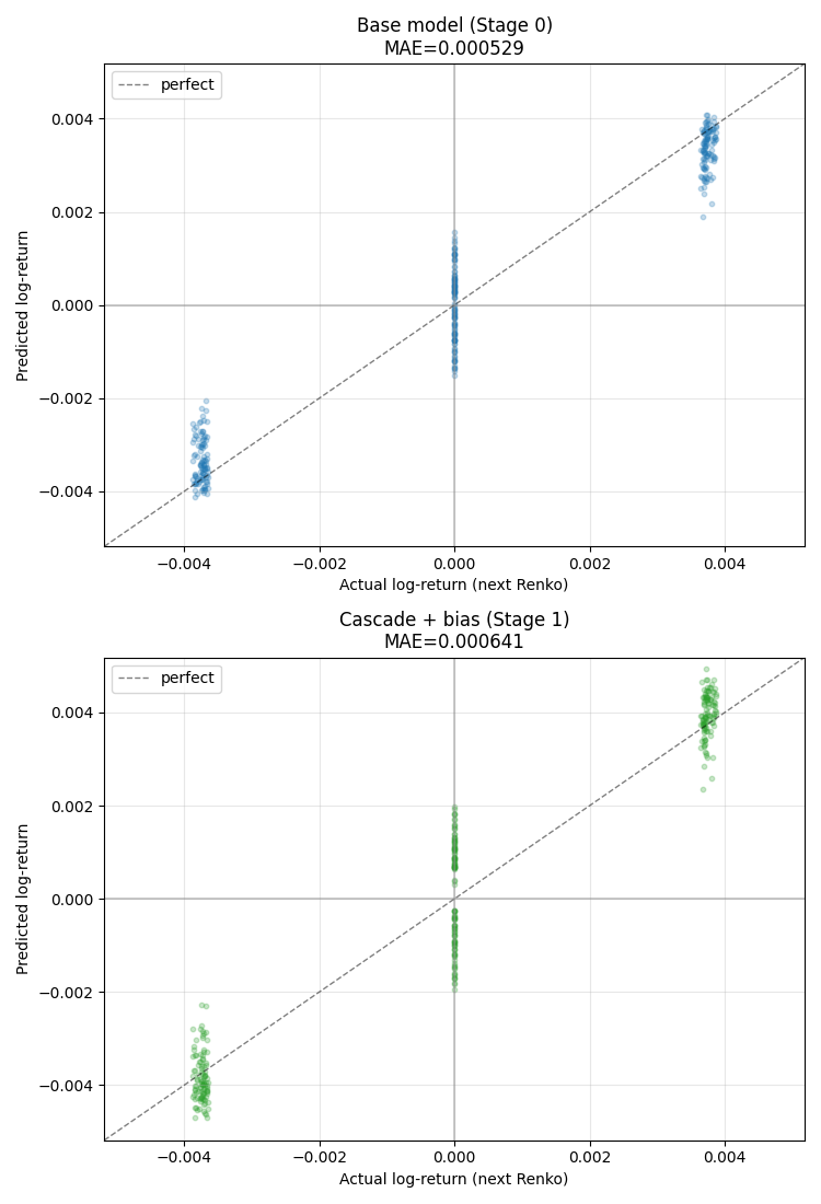
In each cluster, you can see how the model distributes its predictions. In the right cluster (actual = +brick), the predictions are grouped above zero and extend toward the "perfect" diagonal. In the left cluster (actual = -brick), conversely, the predictions are below zero. After the cascade and bias correction (lower plot), the spread of the predictions is wider, but the cluster centers are closer to the diagonal.

The following chart is the most important one from a practical standpoint. The green forecast line almost perfectly coincides with the black line representing the actual price of the next bar across all of the last 300 Renko bars.

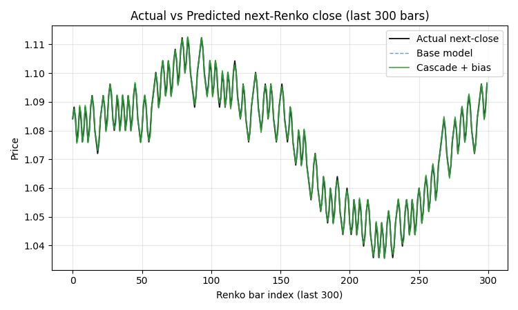
The model's misses are the points where the green line deviates from the black line by exactly one brick_size (about 40 pips on the chart). This behavior is by design: if the model correctly predicts the direction, the prediction lands exactly at the point ±1 brick from the current price; if it is wrong, it misses by exactly one brick.

The residuals after the cascade remained centered at zero (mean = -7e-5, practically zero) with σ ≈ 0.0008. The distribution is symmetrical, with no heavy tails and no apparent skew toward either side.

Summary of metrics for the base model versus the final cascade composition with bias correction: OOF-MAE decreased from 0.001306 to 0.001262 (a 3.35% improvement), OOF-RMSE from 0.001656 to 0.001605, and R² increased from +0.7132 to +0.7183. Direction accuracy remained virtually unchanged (65.15% vs. 64.77%), while residual σ decreased from 0.001655 to 0.001630.

The identified biases were as follows: global_bias = -4.7e-5, bull_bias = -3.1e-4, bear_bias = +2.2e-4 — that is, the model systematically underestimated bull movements and overestimated bear movements.

Direction accuracy decreased slightly after the cascade, but this is offset by an improvement in MAE and more accurate confidence intervals. In trading, what matters most is not predicting the direction of the market, but accurately assessing the magnitude of the move and its uncertainty — and that is precisely what the cascade improves.

Conclusion

We built a complete Renko-bar forecasting pipeline using CatBoost regression and multi-stage error correction. Formulating the problem as a regression rather than a classification task yields a continuous forecast with an uncertainty estimate, which is more important than a binary signal for making decisions about position size and filtering out weak price movements. A cascade of residual models with honest OOF residuals via TimeSeriesSplit makes it possible to iteratively refine the forecast without overfitting, while shrinkage and stronger regularization at the residual stages protect against fitting noise. Conditional bias correction compensates for systematic asymmetry between bull and bear forecasts, and the degradation guard automatically disables the correction if it worsens the metric.

On daily EURUSD data, the system showed an OOF-MAE of 0.001262 and a direction accuracy of 64.8% — robustly above random guessing. On shorter timeframes (M5, M15, H1), where the number of Renko bars over the same period is tens of times greater, the cascade is expected to converge more deeply (5–7 stages instead of two), with correspondingly more accurate forecasts. Possible directions for further development include adding quantile regression for asymmetric confidence intervals, learnable per-stage shrinkage via OOF-MAE optimization, stacking stage predictions using linear regression instead of simple summation, and investigating how the optimal cascade depth changes as the forecast horizon increases. The complete system code — the files RenkoRegressorCascade.py and RenkoBattle_EURUSD_D1.py — is included with this article. Running it requires Python 3.10+, MetaTrader 5 with the MetaTrader5 package installed, and the catboost, scikit-learn, pandas, and numpy libraries.

File	Description
RenkoRegressorCascade.py	Main module: building Renko bars, generating features, a cascade of CatBoost residual models with OOF validation, and conditional bias correction
RenkoBattle_EURUSD_D1.py	Production script: connects to MetaTrader 5, loads EURUSD D1 data, trains/loads the model, and generates a trading signal with calculation of position size, SL, and TP