Uncertainty as a Model (Part 6): Multiple Regression and Diagnostics

Table of Contents

1. Introduction
2. Multiple Regression
• Formal Notation
• Matrix Notation
3. Statistical Analysis
• Residual Analysis
• EDA Methods
• CDA Methods
4. Methods for Working with Regressors
5. Applications of Regression
6. Practical Examples
• Example 1: Nonlinear Trend
• Example 2: Days of the Week
• Example 3: News Days
7. Conclusion
8. Attached Files

Introduction

In real-world trading, an asset rarely moves on its own. By attempting to explain price movements based solely on past price data or a single related index (as in the case of simple regression), a trader risks encountering the "omitted variables" problem. The market is multifaceted: an asset's price is influenced simultaneously by interest rates, broad-market volatility, and many other factors. Ignoring these factors turns the model into a "curve-fitting" exercise that falls apart at the first change in market conditions.

This article focuses on the transition to multiple regression — a tool that allows us to account for the influence of several deterministic factors at once. We will explore how to isolate the contribution of a specific regressor and avoid the pitfalls of multicollinearity, which occurs when variables overlap and distort the signal. Instead of searching for a single "magic" variable, we will learn to build a balanced, multifactor framework that provides a deeper understanding of market structure than a simple correlation between two instruments.

Multiple Regression

The dependent variable is typically influenced by a combination of factors. Analyzing them separately using simple regression yields misleading results, especially if the regressors are correlated with one another. In this case, the influence of unaccounted-for factors is transferred to the random component, thereby depriving the model of its key properties. The parameter estimates become biased: they systematically overestimate or underestimate the true degree of influence of the variables.

However, this does not mean that the model should include as many predictors as possible. Redundant variables that have no real connection to the process under study reduce the model's accuracy and lead to incorrect conclusions.

Thus, the task is to build a multiple regression model that accounts for the simultaneous influence of several factors. To do this, we need mathematical tools to compare different specifications. This will allow us to select the set of regressors that best describes the relationship under study and is suitable for solving practical problems.

Formal Notation

Mathematically, the multiple regression model is expressed as follows:

Yt = B1 * X1,t + ... + Bk * Xk,t + C * Et, where

• Yt is the dependent variable (the process under study) at times t = 1, ..., n.
• Xi,t — the independent variable (regressor) indexed by i at time t.
• B1, ..., Bk, C — model parameters (constants) to be estimated.
• Et — standard Gaussian noise with distribution N(0, 1) at time t.

Compared to simple regression, two important qualitative changes occur here:

1. Unified notation. We no longer specify the intercept (constant term) separately. This role is fulfilled by the coefficient B1, provided that the first regressor X1,t is identically equal to one. This approach significantly simplifies the analytical calculations.
2. The requirement for the absence of multicollinearity. It is assumed that no single regressor can be expressed as a linear combination of the others. While in simple regression this condition simply meant that the independent variable could not be a constant, in a multiple regression model it becomes a critical requirement for the data structure.

The fundamental condition remains the same: for correct parameter estimation, the random component Et must be Gaussian white noise.

As with simple regression, a distinction is made between specifications with deterministic regressors and those with stochastic regressors. Models with stochastic variables, in turn, are classified as either exogenous or endogenous. We already touched on this classification in the introductory article, but now the structure of multiple regression will allow us to examine these differences in greater depth.

For now, the main discussion will focus on the version with deterministic regressors. This is necessary to avoid overloading the text with an excessive number of new concepts and to focus on the basic mechanics of the model. However, we will definitely return to stochastic models, since without them, regression analysis would lose much of its practical value for trading applications. Moving on to these models will allow us to work with more complex and realistic market relationships.

As in simple regression, we obtain the estimates b₁, …, bₖ for B1, ..., Bk using the ordinary least squares (OLS) method. The parameter C is estimated using the unbiased variance estimator: (c² = (e₁² + ... + eₙ²) / (n - k)).

We will omit the intermediate calculations for the coefficients b₁, ..., bₖ and move directly to the final results. To do this, we need to use the tools of linear algebra.

Matrix Notation

The use of vectors and matrices is the accepted standard for describing regression models. This notation not only makes formulas more concise and intuitive, but also aligns directly with the logic of most statistical software packages and data analysis libraries. Let's review the basic definitions:

• A matrix is a rectangular table of numbers whose dimensions are determined by the number of rows and columns.
• A vector is a special case of a matrix consisting of a single column (column vector) or a single row (row vector). In the specialized literature, the term "vector" most often refers to a column vector; however, to avoid errors, it is always a good idea to clarify the dimension based on the context of the specific problem.
• A scalar is an ordinary number.

Let's introduce the following notation to write the formula in a compact form:

• X is a matrix of regressors with n rows and k columns; the entry at the intersection of row t and column i is the value of the regressor Xi,t.
• y is a column vector of values of the dependent variable Yt.
• b is a column vector of the parameter estimates bᵢ to be determined.

Here, the subscript t (time points) takes values from 1 to n, and the subscript i (factor numbers) takes values from 1 to k. Using this notation, the solution to the ordinary least squares (OLS) problem for the coefficient vector b is as follows:

b = (X^T * X)^-1 * X^T * y, where:

• X^T is the transpose of X.
• (X^T * X)^-1 is the inverse of the product of the transposed matrix and the original matrix.
• The asterisk symbol denotes matrix multiplication.

This formula is fundamental. This is precisely the formula that any software evaluates when we fit a regression model. It is important to understand that the existence of the inverse matrix depends directly on the aforementioned condition of no multicollinearity: if the regressors are linearly dependent, the calculations will be impossible.

Statistical Analysis

Analysis in multiple regression is an iterative process. It is difficult to represent this process as a linear sequence of steps, as was done for simple regression. In practice, we constantly modify the model specification: adding new factors, removing statistically insignificant ones, or transforming existing ones. Every change to the set of regressors creates a new model that requires a full cycle of diagnostic checks. Nevertheless, it is possible to identify a set of standard analytical procedures — the “building blocks” that make up the research algorithm.

Residual Analysis

The methods for analyzing residuals carry over from simple regression to multiple regression without substantial changes. This means studying the residuals as a time series in their own right, without considering their relationship with the regressors. As a reminder, these include:

• Visual analysis: a plot of residuals over time.
• Distribution assessment: empirical probability density function (EPDF) plots and QQ plots to compare the residuals with a normal distribution.
• Autocorrelation analysis: plotting a correlogram and conducting the appropriate statistical tests.
• Formal tests: testing for normality of the distribution and for stability of the mean and variance (absence of heteroscedasticity).

Of course, in multiple regression analysis, there are also specific diagnostic methods designed to examine the relationships between variables.

EDA Methods

A correlation matrix is a square matrix containing the correlation coefficients between all pairs of regressors and between each regressor and the dependent variable. If a model includes a constant term (the first regressor equals one), it is usually excluded from the matrix because its correlation with other variables is zero. The main diagonal always consists of ones. The matrix is often visualized as a heatmap, where color intensity reflects the strength of the association and additional labels indicate the significance level (p-value). The matrix is necessary for the initial selection of factors: ideally, the correlation between a predictor and the dependent variable should be high, while the correlation among the predictors themselves should be minimal.

Scatter plots. Compared to simple regression, the range of visualization tools available here is significantly broader. A simple "regressor versus residuals" plot loses some of its meaning, since the residuals now reflect the combined effect of all the factors. Other types of plots take center stage:

• Pairwise scatter plots. These plot the regressors against the dependent variable and against one another. They supplement the correlation matrix, making it possible to visually identify nonlinear relationships and outliers.
• Partial regression plots. They are constructed separately for each regressor and allow us to isolate its individual contribution to the model while accounting for the effects of the other factors.
• Forecast vs. Actual. A scatter plot of forecast values versus actual values. The closer the cloud of points is to the line Y = X, the higher the model's predictive power.
• Predicted values vs. residuals. A critically important plot for visually checking homoscedasticity (constant variance) and identifying hidden patterns that the model was unable to "extract" from the data.

The following metrics are used to quantitatively assess the quality of the model:

• R-squared (coefficient of determination). This metric compares the current model to a "baseline" regression on a constant alone. Mathematically, it represents the proportion of the dependent variable's variance that can be explained by the selected predictors. If the model includes a constant, the R-squared value ranges from 0 to 1: the higher it is, the more accurately the model describes the historical data. In simple regression, this statistic is exactly equal to the square of the correlation coefficient between the dependent variable and the single predictor. It is important to note that in the absence of an intercept (constant term), the standard interpretation of R-squared is no longer valid.
• Adjusted R-squared (Adjusted R-squared). The standard R-squared has a significant drawback: it increases whenever a new predictor is added, even if that predictor does not provide any useful information but merely introduces noise. The adjusted coefficient offsets this effect by imposing a "penalty" for increasing the number of parameters. Formally, it is calculated by replacing the biased estimate of the variance of the residuals with an unbiased one (taking into account the number of degrees of freedom). This makes it a more reliable tool for identifying the optimal set of factors.
• F-statistic. R-squared alone does not tell us whether the result is statistically significant or merely due to chance in the sample. The F-statistic is used to address this question, and its value is directly related to R-squared. Since the distribution of this statistic is known, it allows us to test the null hypothesis regarding the statistical significance of the model as a whole.

Checking for multicollinearity among the predictors. In the case of exact linear dependence, the matrix (X^T * X) is singular, so ordinary least squares (OLS) cannot be applied. However, even when the dependence is strong but not exact, the practical value of the model decreases sharply. The variance inflation factor (VIF — Variance Inflation Factor) is used to assess the degree of multicollinearity. It is calculated separately for each regressor based on the coefficient of determination of the model in which that regressor serves as the dependent variable and all others as independent variables. VIF takes values of 1 or higher: the higher the value, the stronger the linear dependence of that factor on the others. VIF = 10 is generally considered the critical threshold. Exceeding this threshold indicates that the regressor is redundant and is a prime candidate for exclusion from the model. It is important to understand that when at least one variable is removed, the VIF values for all remaining factors are recalculated, since the structure of the relationships within the X matrix changes.

Checking observations for outliers. Individual outliers can have a decisive influence on the model's coefficients, effectively "pulling" the regression toward themselves. Cook's distance is used to quantify this effect. This metric measures the extent to which a specific observation influences the results of the analysis. It shows how much the regression coefficients would change if this data point were excluded from the sample. High Cook's distance values indicate that the observation is an influential outlier that requires careful examination. This stage of analysis is critically important for trading. Financial time series are characterized by "heavy tails" — rare but extreme price movements. Unlike technical measurement errors in physics, such outliers convey important market information and cannot simply be ignored. Analyzing Cook's distance helps determine whether the profitability of a trading strategy is the result of a small number of random price movements in the past.

CDA Methods

Once we have visually assessed the model and selected the regressors, we need to proceed to rigorous statistical hypothesis testing. The purpose of this stage is to confirm that the patterns identified are not mere coincidences and that the model is mathematically sound. Residual diagnostics (carried over from simple regression) — let’s review the main tools:

• Ljung–Box test: checks for the presence of "memory" (autocorrelation) in the residuals. If there is structure in the residuals, it means the model did not extract all the useful information from the data.
• Jarque–Bera test: checks residuals for normality (analysis of kurtosis and skewness). Deviations from normality can severely distort the results of t-tests.
• Pettitt test: used twice — on the residuals themselves (to test the stability of the mean) and on their absolute values (to test the stability of the variance). Any "break" in these measures over the historical period indicates instability in the trading system.

New specification tools — the tests we introduced earlier are critically important for multiple regression:

• The Breusch–Pagan test: the primary tool for diagnosing heteroscedasticity.
• Ramsey's test: checking whether the functional form is correctly specified.
• F-test: an overall assessment of the model's significance.

Let's take a closer look at them.

Breusch–Pagan test (Breusch–Pagan test). The classical model assumes that noise has constant variance. However, in financial markets, this condition is often violated: as volatility increases or the market regime changes, the dispersion of the model’s residuals may increase or decrease. This phenomenon is called heteroscedasticity. The Breusch–Pagan test allows us to formally test whether the variance of the error term depends on the values of the regressors.

The method involves fitting an auxiliary regression. We take the squared residuals from the main model and try to explain them using our regressors. If the regressors do not explain the magnitude of the squared residuals at all, then the variance is random and constant (homoscedasticity). If, however, a relationship is found, it means that the variance changes systematically with market factors. Mathematical implementation: the following auxiliary model is estimated: eₜ² = g₁ * X1,t + ... + gₖ * Xk,t + Ut. The test statistic is calculated as follows: LM = n * R²aux, where n is the number of observations and R²aux is the coefficient of determination for the auxiliary regression. The resulting value follows a chi-square distribution, which makes it possible to calculate the p-value.
Interpretation for traders:

• A low p-value (usually less than 0.05): the null hypothesis that the variance is constant is rejected. The model requires further refinement (for example, switching to volatility modeling using a model such as GARCH or using robust standard errors).
• A high p-value: the variance is stable, and the model correctly estimates forecast uncertainty.

If the Breusch–Pagan test confirms heteroscedasticity, this does not necessarily mean that the model should be discarded. The coefficient estimates remain unbiased, but their standard errors (and, consequently, their t-statistics) become incorrect. In trading, this creates a risk of treating an indicator's effect as statistically significant when it is actually just a consequence of a spike in volatility. To address this problem without changing the model's structure, robust standard errors are used — most commonly White's estimates (White standard errors) or heteroscedasticity-consistent standard errors (heteroscedasticity-consistent errors). To avoid making the article overly long, we will leave a detailed discussion of this topic for a possible future article.

Ramsey test (RESET). By definition, linear regression looks only for linear relationships. However, in financial markets, a factor's effect may strengthen or weaken depending on its magnitude. The Ramsey test (Regression Specification Error Test) allows us to determine whether the chosen linear form is adequate or whether the model suffers from a specification error. Test logic: If there is hidden nonlinearity in the data, then our model's predicted values (Ypred) will correlate with this unaccounted-for component. The test proposes "extending" the model by adding the predicted values raised to the second, third, and higher powers as new regressors: Y = B*X + g₁*(Ypred²) + g₂*(Ypred³) + ... + E.

If the coefficients for these new variables (g₁, g₂, ...) turn out to be statistically significant, it means that the original linear model was incomplete and failed to capture the full pattern. Interpretation for the trader:

• Low p-value: The model has failed to capture the form of the relationship. A linear approximation is too crude in this case. It is worth trying to add logarithms, squared indicator values, or their interaction terms.
• High p-value: The linear specification is adequate, and adding nonlinear terms will not improve the fit of the model.

F-test for overall regression significance. While the t-statistic tests each coefficient individually, the F-test evaluates the model as a whole. The idea behind the test: The F-statistic compares our model's explanatory power with that of a constant-only regression, which simply returns the mean of the series. For a trader, this is the first "coarse filter": if a model fails the F-test, there is no point in analyzing its individual indicators.

• Low p-value: the model is statistically significant. At least one of the selected factors does indeed influence the result, and it makes sense to use these variables together.
• High p-value: the model is useless. Even if the R-squared value seems acceptable, the test indicates that such a result could have been obtained by chance using a set of random numbers.

Methods for Working with Regressors

When a standard linear model does not perform well enough, we can transform the factor space. The most obvious approach is to add new regressors and remove those that are not statistically significant. Let's outline the main alternative approaches.

Dummy variables (Dummy variables). Not all factors can be expressed as a number. Binary variables (which take values of 0 or 1) are used to account for qualitative characteristics or events.
Example: accounting for the day of the week, the trading session (Asia/Europe), or the release of important news. The variable takes the value 1 when the event occurs and 0 at all other times. Important: If we use N categories (for example, 4 trading sessions), we must include N - 1 variables in the model to avoid the "dummy variable trap" (perfect multicollinearity with the constant term).

Nonlinear transformations. If the Ramsey test indicates a specification error, that is a reason to introduce nonlinearity.

• Polynomials: Adding squares or cubes of the regressors (X², X³) allows you to model parabolic relationships — for example, when an indicator's effect becomes stronger as it reaches extreme values.
• Logarithms: Converting to logarithms (log(X), log(Y)) often helps stabilize the variance and shift from absolute changes to relative (percentage) changes, which is more natural for price quotes.

Effects of interaction terms. Sometimes the effect of one factor depends on the state of another. In a linear model, this is accounted for through the product of the regressors: Y = B1 * X1 + B2 * X2 + B3 * (X1 * X2) + E. Example: The impact of an interest rate on a currency can vary depending on whether stock market volatility is high or low. The interaction term will allow the model to "understand" this context.

Multicollinearity. If VIF has identified a strong linear relationship between the factors, the problem can be addressed using the following methods:

• Reducing redundancy: removing one of a pair of correlated predictors.
• Variable transformation: the shift from absolute price values to price changes (returns), spreads, or relative differences.
• Principal component analysis (PCA): transforming a set of correlated factors into a new set of orthogonal (uncorrelated) variables while preserving as much useful information as possible.

After changing the composition or form of the predictors, the model is re-estimated, and the EDA and CDA steps are repeated. It is precisely this cyclical nature that makes creating a high-quality trading system a complex, multi-step process. You can't just "feed" raw data into a statistical package and expect a ready-made trading holy grail. Automation handles the computationally intensive steps; model design remains the researcher's responsibility. Here, a trader’s intuition and understanding of the market context must be harmoniously combined with the strict discipline of statistical methods. Only such a synthesis makes it possible to distinguish genuine market inefficiency from a random coincidence in the numbers.

Applications of Regression

As with simple regression analysis, after checking the model’s adequacy, we move on to deriving practical trading benefits from it. Once we are satisfied that the model is correct, two main questions arise: "What factors actually drive the price?" and "Where will the price be at the next point in time?"

Assessing the significance of individual predictors. Even if the model as a whole passed the F-test, that does not mean that every indicator included in it is useful. To assess the contribution of each factor, t-statistics and their corresponding p-values are used.

• The t-statistic is the ratio of the estimated coefficient to its standard error: t = bᵢ / SE(bᵢ). It shows how many times the coefficient's value exceeds its standard error. If the absolute value |t| exceeds the critical value (typically 1.96 for a large sample), the regressor is considered statistically significant.
• The p-value is the probability that the relationship between the regressor and the price is random. In trading, a threshold value of 0.05 is considered the standard. If the p-value is higher, this factor is a candidate for exclusion from the model, since its effect is indistinguishable from noise.

Forecasting. As with the simpler forms of regression discussed earlier, several types of forecasts are calculated:

• Point forecast. In a regression model, a point forecast is the expected value of the dependent variable given specific values of the independent variables. To obtain it, simply substitute the new values of the predictors into the regression equation. The random error term is ignored, since its expected value is, by definition, zero.
• However, a point forecast (a specific number) will almost always be incorrect. It is much more important to obtain an interval forecast that specifies a "range" of expected values. There are two types of intervals:
• Confidence Interval: Shows where the dependent variable will lie, on average. It reflects only the uncertainty inherent in the model itself (the error in estimating the coefficients).
• Prediction Interval: Always wider than the confidence interval, since it includes not only model errors but also the future realization of random noise.

For a trader, it is the prediction interval that matters. It allows you to set appropriate stop-loss and take-profit levels. If the price moves outside the 95 percent prediction interval, it indicates that an extraordinary event has occurred or that the market structure has changed to such an extent that the model is no longer valid.

Practical use of forecasts using price changes as an example. When the dependent variable Yt is the price change (Pt - Pt-1), the results have a directly practical interpretation. In this case, the model provides not just a "fair price," but the expected direction of movement and the degree of confidence in that direction.

1. Point forecast and trade direction. If the predicted value Yt+1 is positive and statistically significant, the model generates a buy signal; if it is negative, it generates a sell signal. However, in trading, it is not just the direction that matters, but also the margin of safety.
2. Using the prediction interval for risk management. The prediction interval gives us the boundaries within which the price will remain with a given probability (for example, 95%).
• Assessing volatility: the width of the interval directly reflects the current level of uncertainty. If the interval widens sharply, the model signals an increase in market noise, which requires reducing the position size.
• Breaching the bounds: if the actual price change falls outside the prediction interval, this is often interpreted as a "structural break event." For a trader, this is a reason to close the position immediately, since the market is not behaving in line with the current model.
3. Signal filtering. Experienced traders rarely enter a trade merely because the forecast is nonzero. A threshold is usually set — for example, the predicted price change must exceed the expected transaction cost (spread + commission) plus a certain amount of "noise." If the model's forecast is below this threshold, no trading decision is made.
4. Incorporating probability. Given the point forecast and the model's standard error, we can calculate the probability that the price will rise by more than a specified amount. This makes it possible to develop strategies with a fixed expected value, entering the market only when the probability of success exceeds, say, 60%.

Practical examples

In this article, we focused on the study of deterministic regressors. In trading practice, these mainly include factors that are directly linked to the time axis. Unlike stochastic (random) indicators, the values of deterministic variables are known to us in advance for any point in the past or future. Below, we will examine three practical scenarios for using such regressors in market data analysis:

1. Nonlinear trend: how to test for and describe a complex price trajectory over time.
2. Accounting for the day of the week: identifying calendar anomalies in asset returns.
3. The impact of news on volatility: assessing changes in market risk when key macroeconomic data are released.

The first two examples continue the analysis of Google's stock performance that began in the previous article. The third example concerns the exchange rate between the euro and the U.S. dollar.

Example 1: Nonlinear Trend (trend.mq5 script)

In the appendix to the previous article, we performed a simple regression of the logarithm of price against time (bar numbers). The result was unsatisfactory: the residuals did not meet the model's requirements. Let's review why it is critically important for a trader that residuals behave like "white noise":

• Model adequacy. If the residuals are structured, the model "fails to detect" some of the patterns. Even if a trend exists, an incorrect specification renders forecasts useless.
• Accuracy of estimates. If the residuals do not have the required properties, we cannot trust the estimated coefficients — they become inefficient.
• Risk of consecutive losses. Instead of a random alternation of small gains and losses, we end up with long streaks of errors in the same direction. For a trading account, this means prolonged drawdowns that are not recouped over the long term.

Let's build a regression model with a linear trend. We obtain a seemingly promising coefficient of determination:

R2 = 0.661

Let's check the model for nonlinearity using the Ramsey RESET test. Results:

F = 255.324, p-value = 0.000

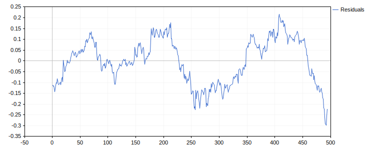
A near-zero p-value clearly indicates a specification error: the linear form is too crude, and nonlinear components need to be added. Following the test's recommendation, let's expand the model by adding the squares and cubes of the bar numbers. With this specification, the coefficient of determination increases as expected:

R2 = 0.831

It would seem that the model has improved significantly. However, a look at the residual plot shatters these illusions. Once again, we see "waves" and prolonged deviations instead of chaotic fluctuations around zero. The correlogram and the Ljung–Box test definitively confirm that the model is unsuitable:

Ljung–Box test result:

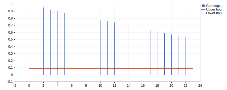
Q = 3,819.190, p-value = 0.000

Conclusion: Even a polynomial trend could not transform the residuals into white noise. We are dealing with a typical case of "spurious regression." Increasing the degree of the polynomial will not fix the problem — the very idea that the price simply fluctuates around a fixed time trend (a TS model) is flawed in this case. An understanding of such problems led econometrics, at the time, to turn to the study of autoregressive models, in which the future depends on the past, rather than solely on the present moment.

Example 2: Days of the Week (days.mq5 script)

When analyzing prices, people often look for calendar patterns — relationships with the time of day, days of the week, quarters, months, or years. However, such patterns often turn out to be nonstationary and contradictory. We will not delve into this topic, as this series of articles provides a general overview of econometrics rather than a detailed analysis of specific effects. Furthermore, econometrics is no substitute for subject-matter expertise: numerical patterns must be supported by an understanding of market dynamics. For example, daily cycles should be explained by the trading session schedule, and quarterly or annual cycles by the tax calendar.

In this example, we will look at how to use dummy variables for the days of the week. The dependent variable is the logarithm of the daily return. Since there are five workdays, four regressors are needed, one for each day from Monday through Thursday: each equals 1 on its designated day and 0 otherwise. On Friday, all four equal 0. Five variables will cause multicollinearity, since their sum will be a constant. The intercept coefficient corresponds to the baseline level, which we have defined as the logarithm of Friday's return. The remaining coefficients indicate how much the dependent variable changes on the other days compared to the baseline level.

The coefficients of determination in the model are low:

R-squared: 0.029
Adjusted R-squared: 0.021

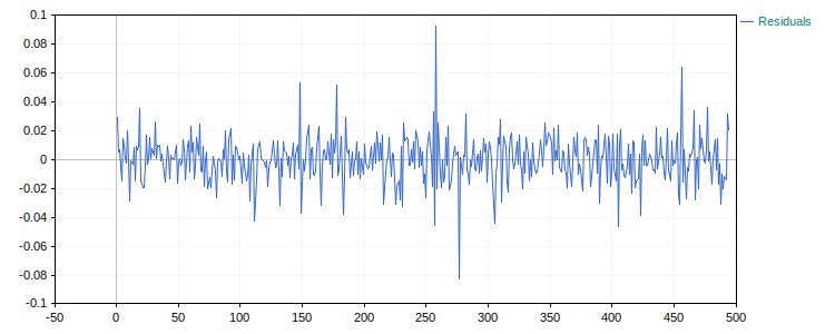
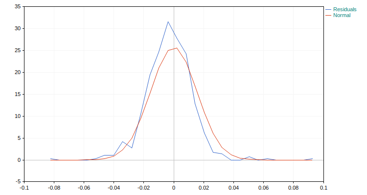
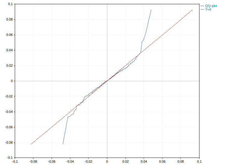
The residuals resemble white noise — this is confirmed by the residual plot, the correlogram, and the Ljung–Box test. The only problem is with the outliers (heavy tails).

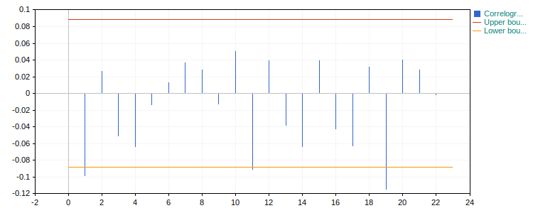
Ljung–Box test result:
Q = 11.124, p-value = 0.348

Checks for normality (EPDF, QQ-plot, and the Jarque–Bera test) reveal deviations, particularly in the tails due to outliers.

Jarque–Bera test result:
JB = 422.580, p-value = 0.000

Let's test the significance of the model as a whole using an F-test for all regressors. The result indicates unexpectedly strong significance (p-value much less than 0.05) for such a low R-squared value:

F-test results for all regressors:
F = 3.668, p-value = 0.006

To get a better understanding, let's evaluate the regressors individually. In the table below, each row corresponds to a single regressor. Only the Thursday regressor, shown in the last row, is significant (p-value < 0.05):

[estimate] [std_error] [t_stat] [p_value] [conf_low] [conf_high]
[0] 0.00083 0.00155 0.53562 0.59246 -0.00221 0.00386
[1] 0.00254 0.00223 1.14056 0.25461 -0.00183 0.00691
[2] 0.00096 0.00218 0.44247 0.65835 -0.00331 0.00524
[3] 0.00058 0.00219 0.26584 0.79048 -0.00372 0.00489
[4] -0.00544 0.00221 -2.45496 0.01444 -0.00979 -0.00109

Overall, the growth is "spread out" across all days except Thursday. There is a noticeable decline in stock prices on Thursdays (estimate = -0.00544) compared to near-zero growth on Fridays (estimate = 0.00083). Let's examine the possible impact of outliers by analyzing Cook's distances. The two largest outliers do not fall on Thursdays; the conservative threshold (4 / n = 0.0081) is exceeded by a moderate amount (max = 0.0727, ratio = 8.98). These values are still well below the critical value of 1, at which the influence of outliers is undeniable.

Cook's distance: max = 0.0727, threshold = 0.0081, ratio = 8.98
outliers in the data (time, return, regressors):
2025.04.09, 9.87%, [1,0,0,1,0]
2025.05.07, -7.77%, [1,0,0,1,0]

Further exploration of this issue goes well beyond the scope of our short article. We need much more complex models, so we will leave the question open. It should be noted, however, that even if there is a real effect, its stability must be continuously verified. The method for identifying structural breaks in models, which we will discuss after autoregression, will be useful for this.

Example 3: News Days (news.mq5 script)

The impact of macroeconomic news on the forex market is undeniable and multifaceted. We will discuss the impact of news on the daily volatility of the EUR/USD exchange rate. We assess the impact of a news release occurring, rather than the specific values of the reported indicators. This allows us to stay within the scope of the article, since news release dates are known in advance (deterministic regressors).

The same set of key macroeconomic indicators is used for each region in the currency pair (the U.S. and the Eurozone). The list includes GDP, the unemployment rate, the inflation index, the central bank's interest rate, and the trade balance. The MetaTrader 5 platform's economic calendar is used to identify days with news releases. In this calendar's API, each event type is identified by a unique ID. To determine this ID, we used the events2file.mq5 script, which writes a complete list of available events (ID and name) for a specified region to a file. The logarithm of the ratio of the daily high to the daily low is used as the dependent variable. The model includes two dummy regressors: the first equals 1 when there is news in the U.S. and 0 when there is none; the second does the same for the Eurozone. The constant corresponds to the return on days when there is no news.

Let's estimate our regression. The model's residuals differ quite substantially from white noise. The normality assumption is particularly severely violated, mainly because of the independent variable we used. For a more accurate analysis, we need to refine the definition of daily volatility, for example by calculating it using intraday bars from shorter time frames. However, our simplified model is quite suitable for a preliminary analysis. Let's see what conclusions we can draw from it. The statistics calculated for the individual model coefficients show that news from the U.S. is statistically significant (a small p-value in the second row), while news from the Eurozone is not (a large p-value in the third row).

[estimate] [std_error] [t_stat] [p_value] [conf_low] [conf_high]
[0] 0.00630 0.00018 34.18283 0.00000 0.00594 0.00667
[1] 0.00166 0.00038 4.39152 0.00001 0.00092 0.00240
[2] 0.00021 0.00037 0.57184 0.56768 -0.00051 0.00093

Let's compare volatility forecasts for days with U.S. news and for days without news. On average, volatility increases by about a quarter when there is news from the U.S. (from 0.63% to 0.80%). This forecast can be used, for example, to adjust a stop-loss order if it is calculated based on daily volatility. It is important to keep in mind, however, that this model requires significant refinement and further development. This is clearly evident from how wide the prediction interval is compared to the confidence interval — too large a proportion of the independent variable’s variability remains unaccounted for in the model (and is treated as noise).

Volatility forecast for U.S. news only, in percentages, at a confidence level of 0.90
Point forecast: 0.80%
Confidence interval: from 0.74% to 0.86%
Prediction interval: from 0.23% to 1.38%
*******************************************************
Volatility forecast for no news, in percentages, at a confidence level of 0.90
Point forecast: 0.63%
Confidence interval: from 0.60% to 0.66%
Prediction interval: from 0.06% to 1.21%

Conclusion

The transition from a one-dimensional perspective to multiple regression is a step toward creating a comprehensive "profile" of a trading strategy. We have seen that adding new factors does not simply complicate the calculations; it allows us to filter out market noise more accurately and identify pure alpha where we previously saw chaos. The main advantage here is the ability to assess how stable an asset's relationship with the outside world is and whether the model is overloaded with unnecessary components.

However, it is important to remember that deterministic regressors are just the foundation. We have learned how to describe static relationships, but the market remains a dynamic system. Understanding how the coefficients distribute weights among the factors provides us with a foundation for the next step — working with stochastic regressors. This will allow us to move from describing static relationships to accounting for market dynamics, using a mathematical framework that is more flexible and better suited to the changing nature of financial instruments.

Attached Files

No.	Name	Description
1	EconometricsA.mqh	A header file containing all the necessary functions (for arrays) to calculate simple regression parameters, plot graphs, and perform statistical tests.
2	EconometricsM.mqh	A header file containing all the necessary functions (for vectors and matrices) for calculating multiple regression parameters, plotting graphs, and performing statistical tests.
3	trend.mq5	A script for calculating and analyzing the cubic trend in log prices.
4	days.mq5	A script for analyzing patterns in logarithms of returns related to the day of the week.
5	news.mq5	A script for analyzing patterns in the logarithms of returns associated with news releases.
6	events2file.mq5	A helper script for displaying all types of news for a specified region.
7	reg2.zip	An archive containing all the files.