How to Implement R/S Analysis and the Hurst Indicator in MQL5

Introduction

If you have ever built a trading system based on historical volatility, you know that feeling of disappointment. The system performs perfectly in the backtester: the Sharpe ratio is high and drawdowns are minimal. You then run it live, and two or three months later, you see the equity curve start to drop just as the market suddenly becomes highly volatile. Classical volatility models failed.

The problem is not with the parameters or overfitting; it runs deeper — it lies in the fundamental assumption underlying GARCH, Black-Scholes, and most classical models: that volatility changes smoothly and randomly, like a standard Brownian motion.

The real market does not behave that way.

In 2014, Gatheral, Jaisson, and Rosenbaum published a paper that revolutionized our understanding of the nature of volatility. They found that the volatility of financial markets is described by fractional Brownian motion with a Hurst exponent H ≈ 0.10. This number is key: it means that volatility is much rougher and more unpredictable than previously thought. Its sample path is nowhere differentiable. That is precisely why any model that assumes volatility is smooth is bound to fail.

This article explains how to turn this mathematical discovery into a working MQL5 indicator. Not a theoretical overview, but a practical tool: a moving-window Hurst exponent estimator that determines the market regime in real time and signals regime changes.

This article systematically examines:

• why classical volatility models are fundamentally flawed;
  
• the theory of fractional Brownian motion and the Hurst exponent;
  
• rescaled range analysis (R/S analysis) — mathematics and implementation;
  
• the complete code for the RoughVolatility_H indicator in MQL5;
  
• signal interpretation and trading applications;
  
• a comparison with classical volatility estimators;
  
• practical diagnosis of the market regime.
  

Why Classical Volatility Models Are Fundamentally Flawed

The classic Black-Scholes model assumes that an asset's price follows geometric Brownian motion with constant volatility. This is mathematically elegant but empirically disastrously wrong. Volatility is not constant — every trader knows that. That is why GARCH was developed.

GARCH and its variants (EGARCH, GJR-GARCH, FIGARCH) allow volatility to change over time. However, they are based on another key assumption: volatility is an integer-order integrated process, meaning it is either stationary (I(0)) or non-stationary (I(1)). Both classes correspond to a Hurst exponent of H = 0.5 or H = 1.0.

Gatheral, Jaisson, and Rosenbaum (2014) conducted an empirical analysis of realized volatility data across several markets: stocks, indices, commodities, and forex. They estimated the Hurst exponent for the logarithm of realized volatility and obtained values of H ranging from 0.05 to 0.20. The average value is about 0.10. This is an order of magnitude lower than all classical models assume.

What does H = 0.10 mean in practice? Volatility movements reverse quickly; volatility spikes are sharp and abrupt — not smooth — and volatility bursts are not anomalies but a systemic characteristic. A model that does not take this into account systematically underestimates risk during calm periods and overestimates resilience during periods of turmoil.

This is precisely what explains why strategies typically fail during market crises: the GARCH model produces conditional volatility that changes too slowly to respond to a sharp spike in actual volatility.

Fractional Brownian Motion and the Hurst Exponent

A standard Brownian motion W(t) has independent increments: knowledge of the past provides no information about the future. Fractional Brownian motion (fBm) is a generalization introduced by Kolmogorov and popularized by Mandelbrot and van Ness (1968) that allows for long-term memory.

Fractional Brownian motion B^H(t) is parameterized by a single number H ∈ (0, 1) — the Hurst exponent:

• H = 0.5 — standard Brownian motion, independent increments, no memory;
  
• H > 0.5 — a persistent process: positive increments are more likely to follow positive ones (a trending market);
  
• H < 0.5 — an anti-persistent process: the increments are negatively correlated across all scales (a mean-reverting market);
  
• H ≈ 0.10 — rough volatility in Gatheral's framework: an ultra-rough process that is close to being nowhere differentiable.
  

A key mathematical property — the scaling law for the variance of the increments of fBm:

//+----------------------------------------------------------------------------+
//| RoughHurst.mq5 — Rough Volatility Hurst Exponent Indicator                 |
//| R/S analysis + OLS regression in log-log space.                            |
//| Estimation of H in a sliding window and classification of market regimes.  |
//| Color coding: Rough, Neutral, Trending.                                    |
//| Copyright 2026, Galym Echanov                                              |
//+----------------------------------------------------------------------------+
#property copyright   "Galym Echanov, www.mql5.com"
#property link        "https://www.mql5.com/en/users/gala_aka_47"
#property version     "1.00"
#property description "Rough Volatility — Hurst exponent (R/S analysis)"
#property description "H < 0.5 → anti-persistent (mean-reverting) mode"
#property description "H = 0.5 → random walk"
#property description "H > 0.5 → persistent (trend) mode"

#property indicator_separate_window
#property indicator_buffers 4
#property indicator_plots   3

//--- Plot 0: Hurst Exponent — colored line
#property indicator_label1  "Hurst (H)"
#property indicator_type1   DRAW_COLOR_LINE
#property indicator_color1  clrOrangeRed, clrDodgerBlue, clrMediumSeaGreen
#property indicator_width1  2

//--- Plot 1: Level H = 0.5 (Random Walk)
#property indicator_label2  "H=0.5 (Random Walk)"
#property indicator_type2   DRAW_LINE
#property indicator_color2  clrSilver
#property indicator_style2  STYLE_DOT
#property indicator_width2  1

//--- Plot 2: Level H = 0.3 (threshold of the Rough zone)
#property indicator_label3  "H=0.3 (Rough Threshold)"
#property indicator_type3   DRAW_LINE
#property indicator_color3  clrOrangeRed
#property indicator_style3  STYLE_DASH
#property indicator_width3  1

//+------------------------------------------------------------------+
//| Input parameters                                                 |
//+------------------------------------------------------------------+

It is precisely this scaling law that forms the basis of R/S analysis: we observe how the rescaled range of a time series scales as the length of the subsample increases, and we estimate the scaling exponent.

Rescaled Range Analysis — R/S Analysis

R/S analysis (rescaled range analysis) was proposed by Hurst in 1951 while studying the Nile floods and was formalized by Mandelbrot and Wallis (1969). This is the most robust nonparametric estimator of the Hurst exponent.

Let r₁, r₂, ..., rₙ be a time series of log returns. For a subsample of length τ, the algorithm consists of four steps. Calculate the mean μ = (1/τ) Σ r_i. Construct the deviation profile Y_k = Σ (r_i − μ). Range: R(τ) = max(Y) − min(Y). Standard deviation: S(τ) = std(r_i). Rescaled range: R/S(τ) = R(τ) / S(τ).

According to the fBm scaling law: E[R/S(τ)] ~ c · τ^H. In logarithmic space: log(R/S) ~ H · log(τ) + const. The Hurst exponent is the slope of a straight line in log-log coordinates, estimated using the ordinary least squares (OLS) method across several scales τ.

The implementation uses logarithmically spaced scales, ranging from the minimum (InpMinScale) to half the window (InpWindow/2). This ensures uniform coverage of the scale range without giving excessive weight to small or large scales.

Indicator Parameters and Buffers

//+-----------------------------------------------------------------------------+
//| RoughHurst.mq5 — Rough Volatility Hurst Exponent Indicator                  |
//| R/S analysis + OLS regression in log-log space.                             |
//| Estimation of H in a sliding window and classification of market regimes.   |
//| Color coding: Rough, Neutral, Trending.                                     |
//| Copyright 2026, Galym Echanov                                               |
//+-----------------------------------------------------------------------------+
#property copyright   "Galym Echanov, www.mql5.com"
#property link        "https://www.mql5.com/en/users/gala_aka_47"
#property version     "1.00"
#property description "Rough Volatility — Hurst exponent (R/S analysis)"
#property description "H < 0.5 → anti-persistent (mean-reverting) mode"
#property description "H = 0.5 → random walk"
#property description "H > 0.5 → persistent (trend) mode"

#property indicator_separate_window
#property indicator_buffers 4
#property indicator_plots   3

//--- Plot 0: Hurst Exponent — colored line
#property indicator_label1  "Hurst (H)"
#property indicator_type1   DRAW_COLOR_LINE
#property indicator_color1  clrOrangeRed, clrDodgerBlue, clrMediumSeaGreen
#property indicator_width1  2

//--- Plot 1: Level H = 0.5 (Random Walk)
#property indicator_label2  "H=0.5 (Random Walk)"
#property indicator_type2   DRAW_LINE
#property indicator_color2  clrSilver
#property indicator_style2  STYLE_DOT
#property indicator_width2  1

//--- Plot 2: Level H = 0.3 (threshold of the Rough zone)
#property indicator_label3  "H=0.3 (Rough Threshold)"
#property indicator_type3   DRAW_LINE
#property indicator_color3  clrOrangeRed
#property indicator_style3  STYLE_DASH
#property indicator_width3  1

//+------------------------------------------------------------------+
//| Input parameters                                                 |
//+------------------------------------------------------------------+

The input parameters are divided into three logical groups. Hurst exponent estimation parameters determine accuracy and speed. Regime levels define the interpretation thresholds. Alerts are an optional tool for real-time monitoring.

input group "=== Hurst estimate ==="
input int    InpWindow    = 128; // Calculation window (bars)
input int    InpMinScale  = 8;   // Minimum R/S scale (bars)
input int    InpNumScales = 6;   // Number of logarithmic scales

input group "=== Mode levels ==="
input double InpLevelRW    = 0.5; // Random walk level
input double InpLevelRough = 0.3; // Rough volatility threshold

input group "=== Alerts ==="
input bool   InpAlerts     = false; // Alert on regime change

Four buffers: Hurst exponent values, color indices (DRAW_COLOR_LINE requires a separate buffer for color), a horizontal level at H=0.5, and a horizontal level at H=0.3. The array of log returns, `g_Returns`, is reused across `OnCalculate` calls, which eliminates unnecessary memory allocations on every tick.

//--- indicator buffers
double H_Buffer[];  // values of the Hurst exponent
double C_Buffer[];  // color indices for H_Buffer
double RW_Buffer[]; // horizontal level H = 0.5
double Rg_Buffer[]; // horizontal level H = 0.3

//--- global array of log returns (reused across calls)
double g_Returns[];

//--- previous market regime for alerts
int g_PrevRegime = -1;

Indicator Initialization

//+------------------------------------------------------------------+
//| Indicator initialization                                         |
//+------------------------------------------------------------------+
int OnInit()
  {
//--- Buffer binding
   SetIndexBuffer(0, H_Buffer,  INDICATOR_DATA);
   SetIndexBuffer(1, C_Buffer,  INDICATOR_COLOR_INDEX);
   SetIndexBuffer(2, RW_Buffer, INDICATOR_DATA);
   SetIndexBuffer(3, Rg_Buffer, INDICATOR_DATA);

//--- Drawing begins only after the first full window of data is available
   PlotIndexSetInteger(0, PLOT_DRAW_BEGIN, InpWindow);
   PlotIndexSetInteger(1, PLOT_DRAW_BEGIN, InpWindow);
   PlotIndexSetInteger(2, PLOT_DRAW_BEGIN, InpWindow);

//--- Color scheme for DRAW_COLOR_LINE (index → color):
//--- 0 → Rough/anti-persistent  → OrangeRed
//--- 1 → Neutral              → DodgerBlue
//--- 2 → Trending/persistent  → MediumSeaGreen
   PlotIndexSetInteger(0, PLOT_COLOR_INDEXES, 3);

//--- Short name of the indicator in the window
   IndicatorSetString(INDICATOR_SHORTNAME,
      StringFormat("RoughVol(H)[W=%d, S=%d]", InpWindow, InpNumScales));
   IndicatorSetInteger(INDICATOR_DIGITS, 4);

//--- Warning if parameters are incorrect
   if(InpWindow < InpMinScale * 4)
      Print("RoughVol WARNING: Window too small. Recommended InpWindow >= InpMinScale * 4. "
            "Hurst estimate accuracy reduced.");

   return(INIT_SUCCEEDED);
  }

The Core of the Algorithm is the CalcHurst Function

This is the indicator's main function. It performs a full R/S analysis using OLS regression in log-log space. The logic is divided into three stages: looping over scales, accumulating R/S at each scale, and performing the final regression.

//+----------------------------------------------------------------------------+
//| R/S analysis — estimation of the Hurst exponent                            |
//|                                                                            |
//| Parameters:                                                                |
//|   ret[]  — array of log returns                                            |
//|   start  — starting index in ret[]                                         |
//|   length — length of the analysis window                                   |
//|                                                                            |
//| Returns: H ∈ [0.01, 0.99] or EMPTY_VALUE if an error occurs                |
//|                                                                            |
//| Algorithm:                                                                 |
//|   1. For each scale n (logarithmically spaced from MinScale to N/2):       |
//|      a. Divide the window into non-overlapping subsamples of length n      |
//|      b. For each one: calculate R (range) and S (standard deviation)       |
//|      c. Calculate the average log(R/S) for a given n                       |
//|   2. OLS regression: log(R/S) ~ H * log(n) → H = the slope of the line     |
//+----------------------------------------------------------------------------+
double CalcHurst(const double &ret[], int start, int length)
  {
//--- Boundary check
   if(length < InpMinScale * 2)
      return(EMPTY_VALUE);

   double logN_min = MathLog((double)InpMinScale);
   double logN_max = MathLog((double)(length >> 1)); // log(length / 2)

   if(logN_max <= logN_min + 1e-10)
      return(EMPTY_VALUE);

//--- Accumulators for linear regression in log-log space
   double sumX  = 0.0, sumY  = 0.0;
   double sumXY = 0.0, sumX2 = 0.0;
   int    nPts  = 0;

//--- Loop over logarithmically spaced scales
   for(int s = 0; s < InpNumScales; s++)
     {
      //--- Scale n: from InpMinScale to length/2 (log-uniform)
      double alpha = (InpNumScales > 1) ? (double)s / (InpNumScales - 1) : 0.0;
      int    n     = (int)MathRound(MathExp(logN_min + (logN_max - logN_min) * alpha));
      n = MathMax(InpMinScale, MathMin(length >> 1, n));

      //--- Number of non-overlapping subsamples of length n
      int numSubs = length / n;
      if(numSubs < 1)
         continue;

      double logRS_acc = 0.0;
      int    logRS_cnt = 0;

      //--- Loop over subsamples
      for(int sub = 0; sub < numSubs; sub++)
        {
         int i0 = start + sub * n;

         //--- Mean return in the subsample
         double mu = 0.0;
         for(int i = 0; i < n; i++)
            mu += ret[i0 + i];
         mu /= n;

         //--- Cumulative deviations, range R, and variance
         double cumDev = 0.0;
         double R_max  = -1e30;
         double R_min  =  1e30;
         double var    =  0.0;

         for(int i = 0; i < n; i++)
           {
            double d  = ret[i0 + i] - mu;
            cumDev   += d;
            var      += d * d;
            if(cumDev > R_max)
               R_max = cumDev;
            if(cumDev < R_min)
               R_min = cumDev;
           }

         double R = R_max - R_min;         // range of cumulative deviations
         double S = MathSqrt(var / n);     // standard deviation

         //--- Accumulate log(R/S) if both values are numerically significant
         if(S > 1e-12 && R > 1e-12)
           {
            logRS_acc += MathLog(R / S);
            logRS_cnt++;
           }
        }

      if(logRS_cnt < 1)
         continue;

      //--- Average log(R/S) for the scale n → regression point
      double logRS = logRS_acc / logRS_cnt;
      double logN  = MathLog((double)n);

      sumX  += logN;
      sumY  += logRS;
      sumXY += logN * logRS;
      sumX2 += logN * logN;
      nPts++;
     }

//--- OLS: slope in log-log space = Hurst exponent
   if(nPts < 2)
      return(EMPTY_VALUE);

   double det = (double)nPts * sumX2 - sumX * sumX;
   if(MathAbs(det) < 1e-14)
      return(EMPTY_VALUE);

   double H = ((double)nPts * sumXY - sumX * sumY) / det;

//--- Clamp to the physically permissible range
   return(MathMax(0.01, MathMin(0.99, H)));
  }

Logarithmically spaced scales. Instead of evenly spaced values (8, 16, 24, ...), exponentially spaced values (8, 13, 22, 36, ...) are used. This ensures uniform coverage in log space and prevents small scales from being overrepresented, as they yield more observation points but less independent information.

Averaging over subsamples. For a scale of n, the window is divided into several non-overlapping subsamples, and R/S is averaged over them. This reduces the variance of the estimate. When n is small, there are many subsamples, and the estimate is stable. When n is large, there are few subsamples — hence the importance of the InpWindow parameter: the larger it is, the more reliable the estimate at large scales.

Numerical stability. The conditions S > 1e-12 and R > 1e-12 prevent division by zero when dealing with degenerate data. The condition |det| > 1e-14 prevents OLS instability when the matrices are degenerate.

Market Regime Identification and Main Calculation Loop

//+------------------------------------------------------------------+
//| Determine the market regime from H                               |
//+------------------------------------------------------------------+
int GetRegime(double H)
  {
   if(H < InpLevelRough)
      return(0);                 // Rough / Mean-reverting
   if(H <= InpLevelRW)
      return(1);                 // Neutral / Random Walk

   return(2);                    // Persistent / Trending
  }

//+------------------------------------------------------------------+
//| Regime name for alerts and logs                                  |
//+------------------------------------------------------------------+
string GetRegimeName(int regime)
  {
   switch(regime)
     {
      case 0:
         return("ROUGH (Mean-Reverting, H < " + DoubleToString(InpLevelRough, 2) + ")");
      case 1:
         return("NEUTRAL (Random Walk)");
      case 2:
         return("TRENDING (Persistent, H > " + DoubleToString(InpLevelRW, 2) + ")");
     }
   return("UNKNOWN");
  }

//+------------------------------------------------------------------+
//| Main calculation function                                        |
//+------------------------------------------------------------------+
int OnCalculate(const int rates_total,
                const int prev_calculated,
                const datetime &time[],
                const double   &open[],
                const double   &high[],
                const double   &low[],
                const double   &close[],
                const long     &tick_volume[],
                const long     &volume[],
                const int      &spread[])
  {
//--- Minimum number of bars required
   if(rates_total < InpWindow + 2)
      return(0);

//--- Size of the log-returns array = rates_total - 1
//--- g_Returns[i] = log(close[i+1] / close[i])
//--- Index 0 = the oldest bar, rates_total-1 = the current bar
   int retSize = rates_total - 1;
   if(ArrayResize(g_Returns, retSize) != retSize)
     {
      Print("RoughVol ERROR: Failed to allocate memory for the returns array.");
      return(0);
     }

//--- Determine the starting bar for recalculation:
//--- On the first run, recalculate everything starting at InpWindow
//--- When updating—only from the last confirmed bar
   int startBar = (prev_calculated <= InpWindow + 1)
                  ? InpWindow
                  : prev_calculated - 1;

//--- Recalculate log returns starting from the required position
//--- Start slightly further back for reliability
   int retFrom = (startBar > InpWindow) ? (startBar - InpWindow - 1) : 0;
   for(int i = retFrom; i < retSize; i++)
     {
      g_Returns[i] = (close[i] > 0.0 && close[i + 1] > 0.0)
                     ? MathLog(close[i + 1] / close[i])
                     : 0.0;
     }

//--- Main calculation loop over bars
   for(int bar = startBar; bar < rates_total; bar++)
     {
      //--- Horizontal Levels
      RW_Buffer[bar] = InpLevelRW;
      Rg_Buffer[bar] = InpLevelRough;

      //--- R/S analysis window: InpWindow log returns ending at bar bar
      //--- g_Returns[bar - InpWindow] .. g_Returns[bar - 1]
      int retStart = bar - InpWindow;

      if(retStart < 0 || retStart + InpWindow > retSize)
        {
         H_Buffer[bar] = EMPTY_VALUE;
         C_Buffer[bar] = 1;
         continue;
        }

      double H = CalcHurst(g_Returns, retStart, InpWindow);

      if(H == EMPTY_VALUE)
        {
         H_Buffer[bar] = EMPTY_VALUE;
         C_Buffer[bar] = 1;
         continue;
        }

      H_Buffer[bar] = H;

      //--- Market regime and line color
      int regime   = GetRegime(H);
      C_Buffer[bar] = regime;

      //--- Alert on a regime change (only on the last bar)
      if(InpAlerts && bar == rates_total - 1 &&
         regime != g_PrevRegime && g_PrevRegime != -1)
        {
         string msg = StringFormat(
            "[RoughVol] %s %s | H=%.4f | Mode: %s",
            Symbol(), EnumToString(Period()), H, GetRegimeName(regime));
         Alert(msg);
         Print(msg);
        }

      //--- Save the current bar's market regime for the next tick
      if(bar == rates_total - 1)
         g_PrevRegime = regime;
     }

   return(rates_total);
  }
//+------------------------------------------------------------------+

Interpreting the Indicator's Signals

The indicator returns a value of H in the range [0.01, 0.99] and colors the line according to the market regime. Colors have specific trading significance.

H Range	Color	Market Regime	Characteristics	Trading Logic
H < 0.3	OrangeRed	Rough / Mean-Reverting	Strong anti-persistence, explosive volatility	Countertrend strategies, mean reversion, pairs trading
0.3 ≤ H ≤ 0.5	DodgerBlue	Neutral / Random Walk	A market with no distinct memory	Refrain from taking directional positions; reduce position size
H > 0.5	MediumSeaGreen	Trending / Persistent	Movements are self-reinforcing; trend persistence	Trend-following strategies, momentum, trend following

The indicator's Network Health is checked by reviewing the history of transitions between market regimes. A shift from the neutral (blue) zone to the Rough zone (red) signals that volatility has begun to behave explosively: upcoming price movements will be sharp, with rapid reversals. It is precisely under such conditions that trend-following systems incur the greatest losses.

A move into the blue zone is also very useful — it often coincides with a preceding trend reversal.

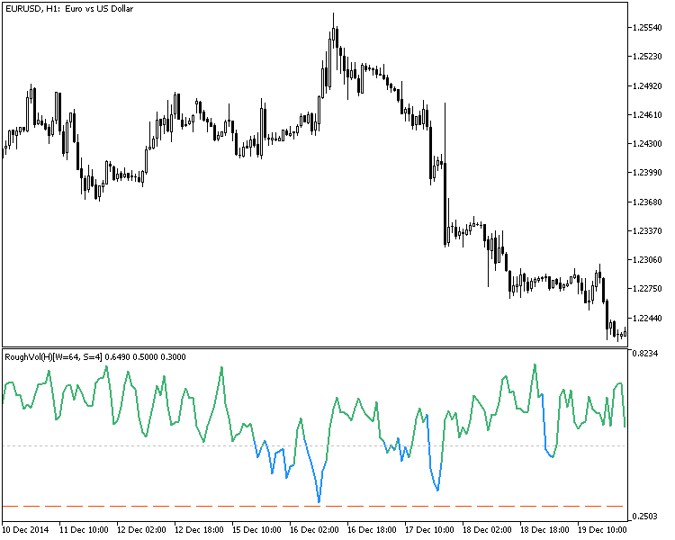
It remains to be seen how informative this feature is for machine learning models, but the screenshots give us hope that CatBoost or XGBoost models will learn to predict reversals more accurately than by chance, using our indicator.

Parameter Selection

The default parameters (Window=128, MinScale=8, NumScales=6) were selected based on the original study by Gatheral et al. and provide a good balance between estimation accuracy and computational load.

Parameter	Default	Recommended range	Impact on the result
InpWindow	128	64–256	A larger window → more stable estimation, but a slower response to regime changes
InpMinScale	8	4–16	A smaller value → more short-term scales and greater sensitivity to noise
InpNumScales	6	4–10	More regression points → a more accurate estimation of H, but a higher computational load
InpLevelRough	0.3	0.25–0.40	Rough-zone threshold: higher → more frequent regime change signals
InpLevelRW	0.5	0.45–0.55	The boundary between neutral and trending market regimes

When trading on scalping timeframes (M1–M5), it is recommended to increase InpWindow to 256–512: short-term noise significantly affects the estimate of the Hurst exponent. On daily bars (D1), you can reduce InpWindow to 64 — the structure is clearer there.

Comparison with Classical Volatility Estimators

The key difference between RoughVolatility_H and ATR, Bollinger Bands, and historical volatility is not that it measures the level of volatility, but that it measures its structure. Two markets may have the same ATR but fundamentally different patterns of price movement.

Tool	What it measures	What it does not capture	Mode of use
ATR	Volatility Level (Bar Range)	Structure: trending or mean-reverting	Position Size, SL/TP
Bollinger Bands	The relative position of the price within a range	Long-term memory of a time series	Breakout/return to the band
Historical Volatility	Standard deviation of returns	Hurst exponent; no information on the market regime	Comparison with Implied Volatility
GARCH	Conditional Volatility with Clustering	H < 0.5; reacts too slowly to volatility bursts	Econometric Risk Modeling
RoughVolatility_H	Hurst exponent — market structure and market regime	Absolute Volatility Level	Choosing a Strategy Type (Trend-Following/Countertrend)

Practical combination: ATR determines the position size and SL/TP levels, while RoughVolatility_H determines the strategy type. When H < 0.3, we use mean-reversion strategies. When H > 0.5, we use momentum strategies. When H is between 0.3 and 0.5, we reduce position size or refrain from entering a trade.

Practical Diagnosis of the Market Regime

In practice, the indicator behaves as follows under various market conditions.

A calm market (low ATR, narrow Bollinger Bands). The Hurst exponent is usually in the range of 0.4–0.6; the line is blue. The market is in a neutral state with no distinct market regime. Exercise caution when entering positions.

A period of high volatility (news events, crises). H drops rapidly to 0.1–0.2, and the line turns red. This is precisely where the roughness of volatility becomes apparent: spikes are sharp and involve reversals. Momentum strategies fail here; countertrend approaches come out on top.

A sustained trend (a directional movement lasting several weeks). H rises above 0.55–0.70; the line is green. This is a rare but valuable state: trend-following systems produce the best results. Important: The green regime often precedes a sharp shift to red when a trend reverses.

A regime change as a trading signal. A shift from the blue zone to the red zone (InpAlerts alert) often occurs before a sharp price movement. It is not the direction, but the very fact of a regime change that serves as a warning of increased risk. This is a signal to review open positions and reduce leverage.

Action Plan in Case of Deteriorating Metrics:

• If H remains consistently below 0.3 for more than 50 bars: switch to countertrend strategies and reduce leverage;
  
• H jumps erratically between zones: increase InpWindow to stabilize it, reduce the trade entry frequency;
  
• H &gt; 0.7 across multiple time frames simultaneously: a rare occurrence; trend-following systems yield the best results, but the risk of a reversal is elevated.

Conclusion: What the Trader Gets

When a trader faces the classic problem — a strategy that works in a backtester but underperforms in the real market during a regime change — the solution lies not in tweaking parameters or using a more complex model, but in understanding the physics of the market. Rough Volatility is not just another moving-average-based indicator. This is a quantitative assessment of the market regime based on the mathematics of fractional Brownian motion.

Three practical uses available immediately after installation.

First, a strategy-type filter. Before each session, we check the color of the line. Red zone — use countertrend tools (RSI overbought signals, return to the Bollinger Bands). Green zone — use trend-following tools (level breakouts, momentum). Blue zone — reduce position size by 50% or wait for a clear signal.

Second, risk management. The market is particularly unpredictable in the red zone. This is a quantitative regime risk metric: reduce leverage, tighten the stop-loss, and lower the number of open positions at any given time.

Third, system diagnostics. If a trend-following system starts to incur losses, the first question is: What is the value of H? If H &lt; 0.3, that does not mean the strategy has failed. This means that the market regime has shifted. Knowing this, you will not over-optimize your strategy; instead, you will simply wait for the market to return to a trending regime.

The indicator requires a sufficient number of bars (Window + several hundred for warm-up) to produce a stable estimate. Extreme values of H < 0.05 or H > 0.95 are most often artifacts of a small sample size rather than genuine signals.

Thus, the trader obtains a reproducible, testable metric of volatility structure — a tool for early detection of market regime changes that enables a shift from meaningless parameter fitting to strategy and risk management based on the market's physical properties.

File name	File description
RoughVolatility_H.mq5	Hurst exponent indicator — R/S analysis, three market regimes, alerts on regime changes