Uncertainty as a Model (Part 5): The Basics of Regression

Table of Contents

1. Foreword
2. Introduction
3. Regression
4. Regression on a Constant
5. Two-Variable Regression
1. Deterministic Regressor
2. Exogenous Regressor
3. Endogenous Regressor
   
6. Conclusion
7. Appendices
8. Attached Files

Foreword

Econometrics, as its name suggests, involves the quantitative analysis of economic data. Once the data have been collected, they must be organized by identifying the real relationships and regularities within them. That is why econometrics exists. Relationships and laws in economics almost never take the form of strictly deterministic dependencies. Therefore, econometrics has its roots in theoretical disciplines such as probability theory, the theory of stochastic processes, and mathematical statistics. At the same time, by its very nature, it is an engineering field in which practical results are more important than adherence to theory. This does not mean abandoning theoretical models. This means treating them as working tools: they should be readily available, available in sufficient variety, and suited to the specific practical task.

Introduction

When moving from looking at charts to developing trading algorithms, the question inevitably arises: how can we formalize the relationship between events? Attempts to find the "golden ratio" or draw a trend line "by eye" often lead us to see a pattern where none exists. Econometrics provides us with the language and tools needed to transform intuitive guesses into rigorous mathematical models.

This article is a practical introduction to regression analysis. First, we'll learn how to distinguish market signals from noise, verify the adequacy of models, and interpret residuals. Instead of blindly trusting return figures, we will learn to spot volatility regime shifts and understand when a mathematical model no longer matches reality. Stock and index quotes are used as examples. We will move from a basic statistical audit to modeling intermarket relationships and obtain a testable basis for trading decisions.

Regression

Regression is the primary tool for data analysis in econometrics. So let's start by defining what we will mean by "data" in this article. Unlike traditional textbooks, let's establish right away that all of our data are time series. That is, specific realizations of discrete-time stochastic processes. We covered them in detail in our previous article, so here we will just recall a couple of points that often cause confusion:

• Terminology: the term "time series" is often used to refer to both the theoretical process itself (e.g., a martingale) and its actual realization (e.g., quotes). Usually, the context makes it immediately clear exactly what is being discussed.
• Confusion of concepts: as a result, people sometimes confuse the theoretical characteristics of a process with their statistical estimates derived from a specific realization. Here, too, context is key.

Let us explain why all the data in this article are treated as time series. The fact is that the specific nature of trading makes it possible to significantly narrow the scope of the study. To address our objectives, there is no need to draw on the full range of econometric tools — for example, methods for analyzing spatial or panel data will not be required in this series of articles. By focusing exclusively on time series, we can explore in greater depth the methods that are directly related to the dynamics of market quotes.

Regression expresses the relationship between one series (the dependent variable) and a set of other series: the independent variables and a stochastic component (noise). The main difference between noise and other types of data is that its realization is fundamentally unobservable. In practice, we work with residuals — the difference between the actual values of the dependent variable and those predicted by the model. Their values depend directly on the model selected. Traders often make the mistake of completely ignoring the residual series. This is incorrect for the following reasons:

• Validation: it is the analysis of residuals that shows how well the model fits the actual data and whether its signals can be trusted.
• Determining process characteristics: the statistical properties of the dependent variable, such as volatility and expected value, are calculated from the residuals. In trading, this has a purely practical significance: without knowledge of these characteristics, it is impossible to construct a correct probabilistic forecast on which decisions about entering or exiting the market are based.
• Detecting a “change point”: a change in the behavior of the residuals is the first sign that the model has stopped working. This means that market conditions have changed and the current parameters are no longer relevant. In this situation, you must either recalculate the model's parameters or abandon the model altogether.

In econometrics, the term “regression” generally refers to linear regression (the word “linear” is often omitted for brevity). Let's not get bogged down in cumbersome general definitions; let's move right on to specific examples of models.

Regression on a Constant

The model is specified by a formula of the form: Yt = A + C * Et, where:

• Yt is the dependent variable (a stochastic process), where t ranges from 1 to n, inclusive
• A and C are model parameters (constants) that must be estimated from a specific realization of Yt
• Et is standard Gaussian noise with zero mean and unit variance at time t

It follows from the formula that Yt is a normally distributed random variable with an expected value equal to A and a standard deviation (SD) equal to C. The maximum likelihood method is used to find the point estimates A and C. When estimating the parameter A, this naturally leads us to minimize the sum of squares: (Y1 - a)^2 + (Y2 - a)^2 + ... + (Yn - a)^2. Hence a (the estimate of A) has the form of the simple arithmetic mean: a = (Y1 + Y2 + ... + Yn) / n. The maximum likelihood estimate of the variance is equal to the mean of the squared deviations of Yt from a. However, this estimate is biased. The unbiased estimate for the square of the parameter C (the variance) is: c^2 = ((Y1 - a)^2 + (Y2 - a)^2 + ... + (Yn - a)^2) / (n - 1).

Despite being extremely simple, this model is highly useful:

• It allows us to model asset price increments (more often, log returns) or a series of returns from trades as a first approximation. This provides a basis for assessing the stability of a trading system.
• It serves as a "baseline" when compared to more complex models.
• It allows us to introduce the minimum set of residual diagnostics needed to check whether they conform to the model.
• This model makes it easiest to demonstrate how to construct a confidence interval for a parameter and the principle of statistical hypothesis testing. This is critically important for understanding whether a result (for example, the average profit) is statistically significant or simply due to chance.

Let's move on to testing the adequacy of the model based on statistical analysis. As we know from the article on mathematical statistics, analytical methods are divided into EDA (exploratory) and CDA (confirmatory). In this context, the first group includes:

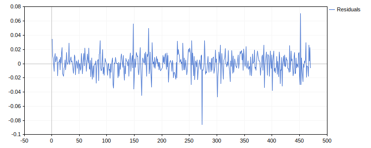
• Plot of residuals over time: allows you to visually identify gross violations of the model assumptions, such as the presence of a trend.
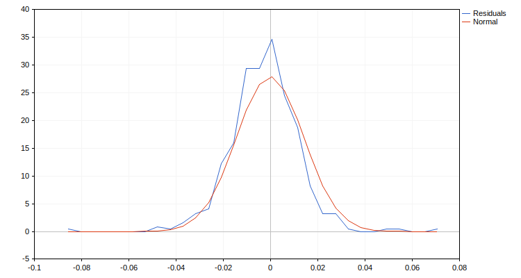
• Histogram of residuals overlaid with the density of a normal distribution: this helps assess symmetry and kurtosis, revealing deviations in the shape of the distribution (primarily in its central region).
• QQ-plot (quantile-quantile plot): a tool for comparing an empirical distribution with a theoretical normal distribution. Unlike a histogram, it provides more information for analyzing the behavior of the "tails" of the distribution.
• Correlogram (ACF plot): a plot of the autocorrelation function for various lags. Used to check the independence of the residuals. The plot typically includes two horizontal lines marking critical levels: values outside these limits indicate the presence of statistically significant dependencies in the residuals.

The second group (CDA) consists of rigorous statistical tests. There is no universal criterion that applies "in all situations": a time series may deviate from the white noise model for various reasons, each of which requires its own testing method. In addition, the choice of test varies depending on the sample size. At this stage, we will focus on the following tools:

• Ljung–Box test: a test for the presence of "memory" (autocorrelation) over a specified range of lags.
• H0: There is no autocorrelation (white noise).
• H1: There is statistically significant autocorrelation in the section under study.
• Jarque–Bera test: a test of distribution shape (analysis of kurtosis and skewness).
• H0: The distribution of residuals follows a normal distribution.
• H1: Significant deviations from normality have been identified.
• The Pettitt test on residuals: testing the stability of the mean.
• H0: The mean of the series remains constant.
• H1: There is a change point in the mean level of the series.
• Pettitt test on absolute residuals: testing the stability of the variance.
• H0: The volatility of the series remains constant over the entire interval.
• H1: A point of abrupt change in volatility (heteroscedasticity) is detected.

Once the model's adequacy has been confirmed, we can move on to its practical application. The main objectives here are to refine the true values of the parameters (since we previously obtained only their statistical estimates) and to develop probabilistic forecasts of the process’s evolution. Although the analytical tools available for this basic model are limited, we can solve a number of important problems:

• Constructing an interval estimate of the true value of parameter A. This makes it possible to determine the range in which the expected value of returns lies at a specified confidence level.
• Testing the hypothesis that parameter A equals zero. This is critically important for a trader, as it allows for statistical confirmation of the presence (or absence) of a positive expected value for a trading strategy or asset.
• Probabilistic forecast for Yt (when t = n + 1). Constructing a prediction interval within which the next value of the series will fall with a given probability. The boundaries of the interval are determined by a quantile of Student’s t-distribution, not of the normal distribution. The reason is that, in practice, we work only with parameter estimates, not with their true values. This once again confirms the need to strictly distinguish between theoretical characteristics and their sample estimates: they are identical only in an infinite sample, which is unattainable in reality.

The appendix to the article presents an MQL5 script that performs all the described checks step by step and displays the final result for a sample of log returns for the selected asset.

Two-Variable Regression

The model is defined by a formula of the form: Yt = A + B * Xt + C * Et, where:

• Yt — the dependent variable (stochastic process) at time points t = 1, ..., n
• Xt is the independent variable (regressor), whose nature determines the methodology for further analysis
• A, B, C — model parameters (constants) to be estimated from the realizations of Yt and Xt
• Et — standard Gaussian noise (white noise) with distribution N(0, 1)

The choice of calculation method depends critically on the type of independent variable. The difference in the complexity of these approaches is fundamental. It is important to understand that this distinction stems from the inherent nature of the data, not from the researcher's choice. Attempting to oversimplify (by ignoring the variable type) will result in inconsistent estimates that are useless — or even harmful — when making trading decisions. We identify three scenarios:

1. Deterministic Xt: the variable is not random (e.g., a time factor or parameters known in advance).
2. Stochastic Xt (exogeneity): the variable is random but is uncorrelated with the noise Et. This implies that the effect of Xt on the system described by Yt is external in nature.
3. Stochastic Xt (endogeneity): the variable is random and correlated with the noise Et. This indicates that Xt is intrinsic to the system under study.

Deterministic Regressor

We will start the study with the simplest scenario. Let us recall a point from an article on probability theory: determinism is not the opposite of stochasticity, but rather a special case of it. This is a degenerate state in which the variance is zero and the entire probability density is concentrated at a single point — the expected value. Nevertheless, in econometrics, this case is classified as a separate category. From a practical standpoint, working with deterministic variables is fundamentally different from analyzing non-degenerate stochastic processes, because it simplifies the requirements for parameter estimation and statistical hypothesis testing.

First of all, you need to make sure that the series Xt is not constant (that is, it contains different values). Otherwise, the move to a more complex model will not happen, and we will effectively remain within the framework of regression on a constant.

The parameters A and B are still efficiently estimated using OLS. The estimate of the noise variance (C^2) is calculated as the mean squared residual, but now n − 2 is used in the denominator.

It is worth mentioning the principle of degrees of freedom here. An initial sample of size n gives us n degrees of freedom. We "use" two of them to estimate the coefficients A and B, so n - 2 remain for estimating the variance. This rule has a rigorous mathematical basis, but for practical purposes it is enough simply to remember it. The number of remaining degrees of freedom is critically important when calculating the p-value in various statistical tests, since it is a parameter of the corresponding distributions (Student’s t, chi-square, Fisher’s F).

The point estimates a, b, and c for the model parameters A, B, and C are as follows:

• b = ((X1 - Mx) * (Y1 - My) + ... + (Xn - Mx) * (Yn - My)) / ((X1 - Mx)^2 + ... + (Xn - Mx)^2), where Mx and My are the mean values of the series Xt and Yt.
• a = My - b * Mx
• c^2 = (e₁^2 + e₂^2 + ... + eₙ^2) / (n - 2), where eₜ = Yt - (a + b * Xt) gives the model residuals.

Let's move on to assessing the model's adequacy for the original data using EDA methods. All the residual analysis tools described for regression on a constant remain valid, but they are supplemented by new, specific plots:

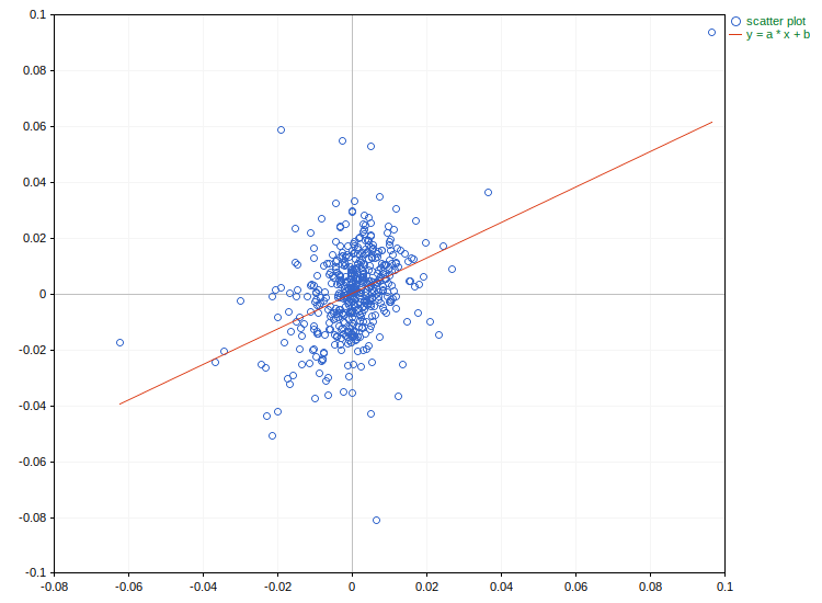
• A scatter plot of Xt against Yt, together with the regression line y = a + b * x. We should see the “cloud” of points concentrated along a straight line. If the data points are scattered randomly, the usefulness of the chosen regressor is questionable. If, on the other hand, the cloud has a distinct curved shape (parabola, logarithmic curve, etc.), this indicates a nonlinear relationship. In this case, to remain within the framework of linear regression, it may be necessary to apply a nonlinear transformation to the original regressor or to switch to multiple regression, where the independent variables will be a set of different transformations of Xt.
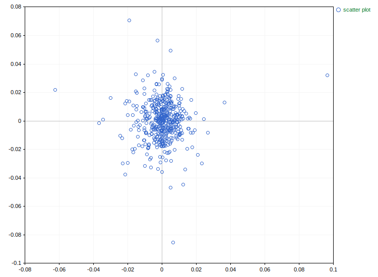
• A scatter plot of the regressor Xt and the residuals eₜ. In an ideal model, there should be no association between them (visually, a uniform cloud). The presence of a trend or a systematic change in the cloud's shape when moving along the Xt axis indicates problems. A widening (or narrowing) of the cloud of points indicates heteroscedasticity — a violation of the condition that the standard deviation of the noise remains constant (C = const). Heteroscedasticity reduces the accuracy of parameter estimates obtained using OLS, although the estimates remain unbiased. To correct the situation, it may be necessary to replace the regressor, transform it, or include additional independent variables in the model.

All statistical tests described for regression on a constant remain valid. However, for simple regression, the analytical toolkit of CDA is expanded to include methods for testing the relationship between the residuals and the regressor, as well as whether the model has been chosen correctly:

• The Breusch–Pagan test: the primary tool for testing for heteroscedasticity. It mathematically confirms (or refutes) the visual suspicions that arose during the analysis of the scatter plots.
• H0: The variance of the error term is constant and independent of the regressor (homoscedasticity).
• H1: The variance of the error term is a function of the regressor (heteroscedasticity).
• Ramsey's test (RESET): checking the correctness of the model's functional form (linearity). It helps determine whether we have overlooked any significant nonlinear components.
• H0: The relationship between Yt and Xt is linear.
• H1: The relationship is nonlinear (the model is misspecified).

The Breusch–Pagan and Ramsey tests inherently require moving to multiple regression, so their discussion will be deferred to the relevant section.

Once the model's adequacy has been confirmed, we can move on to drawing practical conclusions. In the case of simple regression, our toolkit includes:

• Testing the statistical significance of a relationship. We must ensure that the effect of Xt on Yt is sufficiently meaningful for our practical applications and is not merely the result of a random coincidence. To this end, we test the hypothesis that the slope coefficient B is equal to zero using Student's t-test. If the null hypothesis H0: (B = 0) is rejected, the relationship between the variables is statistically supported.
• Constructing a prediction interval. For a new value of the regressor, we calculate the range in which the price will fall with a specified probability. Here, in addition to the uncertainty in the estimate of the mean (as in regression on a constant), there is also uncertainty in the estimate of the coefficient B. This produces a characteristic "hourglass" effect: the prediction interval is narrowest near the mean value of Xt and widens as we move away from it (into the region of new, previously unobserved values of the regressor).

The appendix to the article provides an MQL5 script that implements data analysis for regressing an asset's price on the bar number.

We need to classify the type of the stochastic process Yt. Clearly, it is nonstationary because its expected value is not constant: M(t) = A + B * Xt. However, if we remove this deterministic component (the trend) from the process, we should obtain a stationary series — noise with zero expected value and a constant standard deviation (SD): C.

Processes with this behavior are called trend-stationary (Trend Stationary, TS). This is the most predictable type of nonstationarity: any deviations from the trend line are temporary (the mean-reversion effect). In the section on autoregressive models, we will learn to distinguish them from another, much more "insidious" type — difference-stationary series (Difference Stationary, DS), in which shocks have a cumulative effect.

For now, we will simply note that the class of TS series is considerably broader than the example we have considered: stationary residuals do not necessarily have to be "white noise." They may have their own internal structure (autocorrelation or "memory"), which we will examine in detail in the chapter on autoregressive models.

Exogenous regressor

Let's move on to the case where Xt is a stochastic process. Although in practice we always work with specific numerical series, we must take into account the nature of their origin in order to obtain well-founded forecasts. Unlike a deterministic series, whose future values we know with certainty, a stochastic regressor limits our knowledge of the system's future.

Performing a regression is mathematically meaningless if one of the time series (Xt or Yt) is stationary and the other is not. Otherwise, we would be attempting to express a nonstationary series in terms of a stationary one.

Regressing a nonstationary series on a nonstationary series typically leads to a spurious regression. There are countless examples of thoughtless application of OLS, where processes that are completely unrelated by their nature appear to be statistically linked. The only rare exception is cointegration, which we will discuss after studying autoregressive models.

Therefore, before performing the regression analysis, we must verify that both time series are stationary. To this end, specialized tests (such as ADF or KPSS) are used, along with, if necessary, procedures for transforming the data into a stationary form (detrending or differencing). These topics will also be covered in the section on autoregression.

The need to postpone the details of these procedures highlights a problem with a time-series course. Autoregression cannot be studied without regression, and regression cannot be fully explained without elements of autoregression. The topics in this area are all intertwined, and we will untangle them step by step.

So, let's assume that we have two stationary series. We are considering an exogenous setting, which implies that the effect of Xt on the system is external in nature. From a mathematical standpoint, this means that there is no correlation between the regressor Xt and the model errors Et. Provided this condition is satisfied, the parameter estimates obtained by ordinary least squares (OLS) remain consistent and unbiased.

When performing EDA and CDA for exogenous regression, all of the previously discussed plots and statistical tests of the residuals remain relevant. Specific tools for checking stationarity and cointegration are added to these, and we will study them in detail later. The model’s exogeneity is also subject to rigorous statistical testing; however, we will defer its discussion until the section on multiple regression with endogenous regressors, where the necessary instrumental-variables framework will be introduced. Leaving the theoretical details for later chapters, let's move on to the applied analysis.

As a practical example, we will examine a simplified version of the CAPM (Capital Asset Pricing Model). In the classical version of the theory, calculations are based on excess returns, i.e., returns net of the risk-free rate. However, for the purposes of this article, we will make a simplification that does not distort the essence of the econometric framework: we will estimate a regression directly between the log returns on the stock and the index. We use log returns because they are generally more stationary than prices and simple differences. Let us recall the practical meaning of the parameters in this model:

• Beta (β) reflects an asset's sensitivity to broad market movements. If β > 1, the asset is considered aggressive (it rises and falls more sharply than the index); if 0 < β < 1, it is considered conservative. A negative beta (β < 0) means that the asset moves in the opposite direction to the market.
• Alpha (α) is interpreted as the average return on an asset that is not explained by the index's dynamics. In trading, this is often viewed as an indicator of "skill" in asset selection or of the uniqueness of the asset itself.

An analysis of the residuals from this model will allow us to determine how stable the relationship between the asset and the index is and whether it contains any hidden patterns that would require a shift to more complex models.

The appendix to this article provides an MQL5 script that performs all currently available calculations and generates charts for this example.

Endogenous regressor

If the tests confirm significant endogeneity, this is critical for our OLS estimates: they become biased and inconsistent. The problem is solved by introducing instrumental variables that are correlated with the original regressor but are unrelated to the residuals.

Implementing this method (for example, two-stage least squares (2SLS)) requires a different mathematical framework and, as a rule, involves a transition to multiple regression using matrix notation. To maintain the flow of the discussion, we will return to this topic in the section on multiple regression with endogenous regressors.

Conclusion

Building a regression model is not the end of the analysis, but merely the beginning of an in-depth exploration of the data. We observed that even a statistically significant trend can conceal an autocorrelation trap, while seemingly chaotic noise can contain volatility-regime change points. The main conclusion of this section is that a model is only as valuable as its residuals are clean.

We have learned how to estimate the "alpha" and "beta" of an asset, test hypotheses about the significance of parameters, and construct prediction intervals that account for uncertainty. However, simple regression is only the first step. Recognizing that a single factor is often insufficient to explain the full complexity of market dynamics, we logically arrive at the need to expand our toolkit. In the next section, we will move on to multiple regression and matrix methods to learn how to combine several signals into a single system while maintaining control over quality and avoiding overfitting.

Appendices

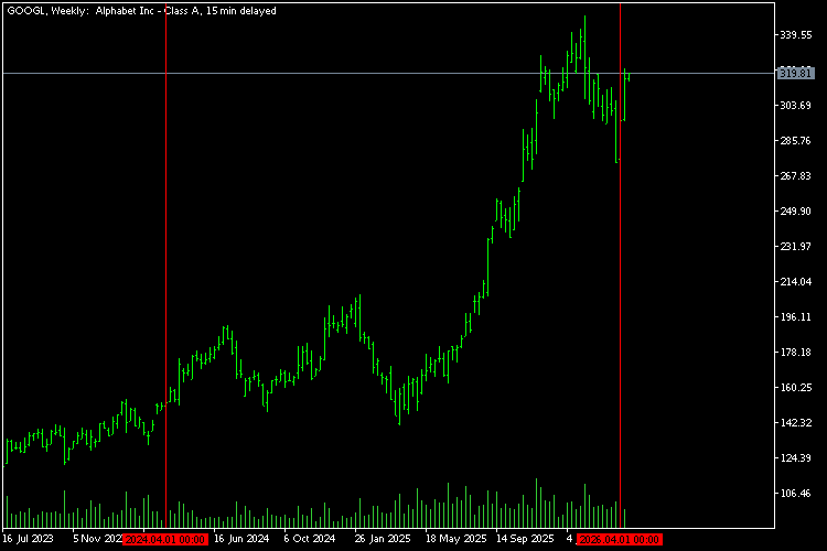
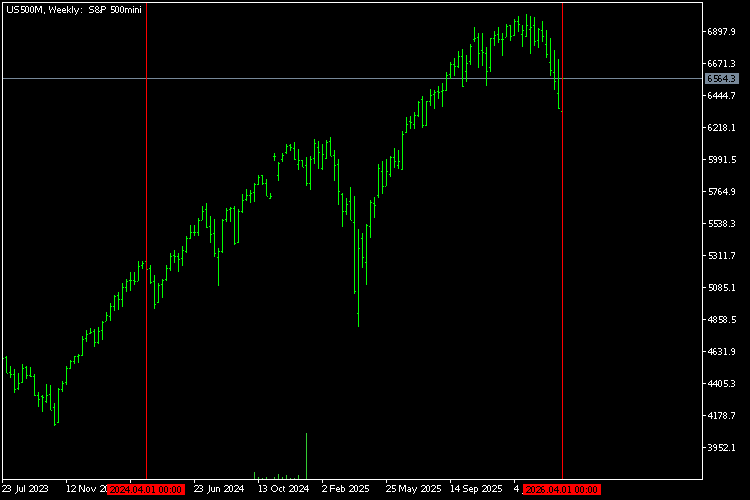
Stock prices of Alphabet Inc. (Google) over the past two years were used as the empirical basis for all three appendices. Class A shares (ticker symbol GOOGL), which have higher liquidity, were selected for the analysis. In the third appendix, the S&P 500 index (symbol US500M in the MetaTrader 5 demo terminal from MetaQuotes) serves as the independent regressor. Below are screenshots of the trading platform showing charts for these instruments. On both charts, the boundaries of the interval under study are marked with red vertical lines. The data for estimating the models were sampled from this interval.

Appendix 1: Regression of log returns on a constant (script reg_const.mq5)

For the analysis, we use log returns (log returns) rather than simple price increments. There are two good reasons for this:

1. Volatility stationarity: in ordinary increments, variance often increases along with price (a stock priced at USD 200 fluctuates more in points than one priced at USD 100). Log transformation levels out this effect, making volatility more homogeneous across the entire historical series.
2. Additivity: log returns are convenient to sum. The sum of daily log returns is exactly equal to the log return over the entire period, which is not true of simple percentage changes.

Log transformation brings the data closer to a stationary process. This is necessary for the proper use of regression.

The script generated the following analysis results:

Number of quotes downloaded for symbol GOOGL: 494

Point estimates of the regression parameters A: a = 0.0013 and C: c = 0.0194

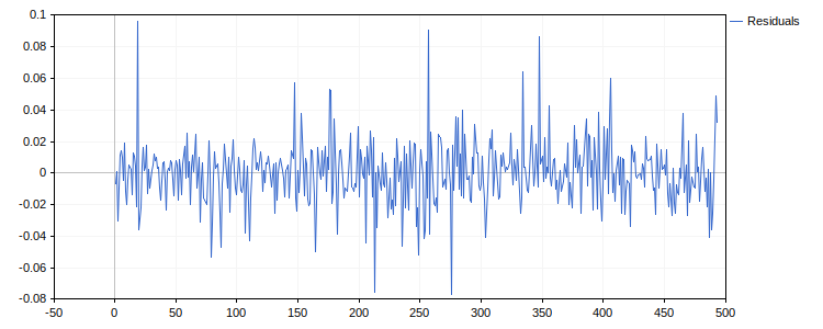
Residual plot: visually, the residual series behaves like white noise. The only major concern is the presence of extreme outliers, which call into question the Gaussian nature of the distribution.

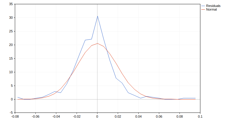
Empirical density: compared to a normal distribution, there is pronounced excess kurtosis (a sharper “bell curve” and a high concentration of data in the center).

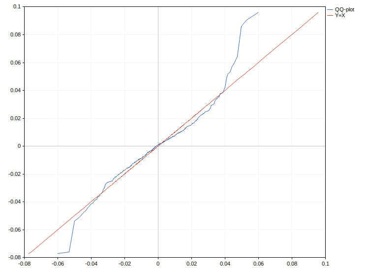
QQ-plot: supports the hypothesis of “heavy tails” in the distribution (leptokurtosis).

Correlogram and the Ljung–Box test: These demonstrate the absence of significant serial correlation in the residuals.

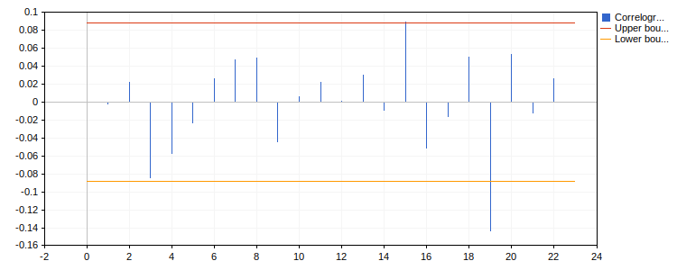
Ljung–Box test result:

Q = 9.319, p-value = 0.502

Jarque–Bera test: quantitatively confirms a statistically significant violation of normality.

Jarque–Bera test result:

JB = 273.992, p-value = 0.000

Stability analysis: Due to deviations from normality, a nonparametric rank-based approach (the Pettitt test) was used. For the residuals: no significant change points (jumps in the mean) were detected.

Pettitt test result:

K = 4256.000, p-value = 0.809, change-point = 264

For the absolute residuals: a statistically significant change in variance was detected. The change point is at the end of October 2024. This change in volatility may be due to a combination of factors: Alphabet's quarterly earnings report, a sharp rise in interest in AI technologies, or uncertainty ahead of the U.S. elections.

Pettitt test result:

K = 9514.000, p-value = 0.022, change-point = 144

Practical application of the model. In addition to analyzing the structure of the residuals, the predictive potential of the parameter A (the expected value of returns) was assessed. Testing the null hypothesis H0: A = 0 against the alternative hypothesis H1: A > 0 yielded p-value ≈ 0.066. This is a borderline result: strictly speaking, we cannot reject the null hypothesis at the standard 5% significance level, but the p-value is close to the cutoff. This gives grounds for cautious optimism, but it requires confirmation using more sophisticated models.

Test H0: A = 0 vs. H1: A > 0 (for regression on a constant) result:

t = 1.508, p-value = 0.066

Interval estimation: The confidence interval constructed for A nevertheless includes negative values (the lower bound is below zero). This confirms that, given the current level of market noise, we cannot guarantee a positive drift.

A between -0.0004 and 0.0030 with a confidence level of 0.950

Interval forecast: the prediction interval constructed for the return on the next bar turned out to be nearly symmetric about zero. The high degree of uncertainty in the forecast is a sufficient reason to avoid opening positions lasting one day based on this very simple model.

Y between -0.0368 and 0.0394 with a confidence level of 0.950

Conclusion: Despite the observed heteroscedasticity and “heavy tails,” the regression on a constant confirms its applicability as a starting point. The analysis clearly indicates the direction for further development: new regressors should not merely describe price dynamics, but also address the specific problems identified — explain when volatility regime shifts occur, mitigate the impact of extreme outliers, and consequently reduce the overall variance of the model's errors in a targeted way.

Appendix 2: Simple Regression with a Deterministic Regressor (script reg_pair_determ.mq5)

In this model, the bar number (time) serves as the independent variable, and the logarithm of the closing price serves as the dependent variable. The use of logarithms is a widely accepted standard, since market trends are often exponential in nature, and applying logarithms allows them to be converted to a linear form.

The script generated the following analysis results:

Number of quotes downloaded for symbol GOOGL: 494

Point estimates of regression parameters A: a = 4.9491, B: b = 0.0014, and C: c = 0.1476

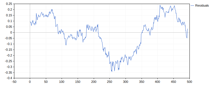
Residual plot: visual analysis of the residuals shows that they are wholly inconsistent with a white-noise model. Instead of random fluctuations, we observe prolonged directional waves.

Autocorrelation: the correlogram has a "comb" shape, with extremely high values (close to one) at all lags.

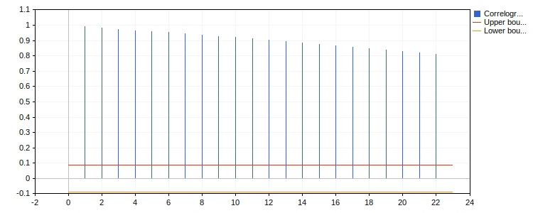
Ljung–Box test: a p-value of 0.000 definitively confirms that the model is untenable.

Ljung–Box test result:

Q = 4579.754, p-value = 0.000

Although the regression coefficients may formally have high t-statistics, such a model is a classic example of a spurious regression. The entire "signal" that we see is due to price inertia, not a functional relationship with time. Further testing and attempts to make predictions using this model serve no practical purpose.

Conclusion: A simple straight line cannot capture price dynamics, even if the trend appears visually obvious. The market trend has a more complex stochastic nature. One solution might be to use piecewise-linear models or adaptive algorithms, but that is beyond the scope of our introductory course. This example serves as an important cautionary note: a visually steep trend slope does not guarantee the quality of a statistical model.

Appendix 3: Regression with a Stochastic Exogenous Regressor (script reg_pair_stohast.mq5)

The script synchronizes data for a stock and an index, estimates the model parameters, and performs a comprehensive audit of the residuals. The calculations were performed under the assumption of exogeneity of the regressor (i.e., no correlation between the index and the model errors). Although this assumption requires separate verification, as we agreed, we will postpone the exogeneity testing procedure until the section on multiple regression.

In this appendix, the format in which the results are presented has been intentionally changed. Instead of a strict division by stage (first all visual analysis, EDA, and then statistical tests, CDA), we grouped the data into thematic blocks: general information, the shape of the residual distribution, their autocorrelation, and the stability of their behavior. This approach allows for a comprehensive evaluation of each property of the model by comparing graphical data with the results of the corresponding calculations. Analysis results:

Number of quotes downloaded for GOOGL stock: 494

Number of quotes downloaded for the US500M index: 514

Number of pairs for regression: 470

Point estimates of the regression parameters A: a = 0.0004, B: b = 0.6360, and C: c = 0.0143

Scatter plots (scatter plots):

The (x, y) graph shows a concentration of data points along the regression line. The visual structure is somewhat smoothed out due to the scale required to display rare outliers.

The plot of (x, residuals) does not reveal any significant patterns, which indirectly confirms the adequacy of the linear form of the model.

Residual plot: visually, the behavior of the residual series corresponds to white noise; however, as in the first appendix, extreme outliers are observed.

Distribution (EPDF and Q-Q plot): These confirm the high concentration of data in the center (“sharp peak”) and heavy tails characteristic of non-Gaussian processes.

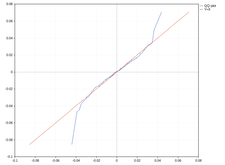
Jarque–Bera test: As expected, it confirms that the residual distribution deviates from normality.

Jarque–Bera test result:

JB = 342.387, p-value = 0.000

Autocorrelation (correlogram and the Ljung–Box test): indicates the absence of serial dependence. This is a critically important result: it means that the index has successfully captured all of the stock’s systematic dynamics.

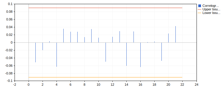
Ljung–Box test result:

Q = 5.331, p-value = 0.868

Stability analysis (Pettitt test):

No change point was found in the mean of the residuals.

Pettitt test result:

K = 3831.000, p-value = 0.858, change-point = 67

For the absolute residuals (for variance) — and this is a key difference from the first appendix — there is also no significant change point.

Pettitt test result:

K = 7062.000, p-value = 0.113, change-point = 220

Practical conclusions:
The model shows that the B (beta) coefficient is highly statistically significant. This confirms the fundamental dependence of the stock’s dynamics on the behavior of the broader market.

Test H0: B = 0 vs. H1: B != 0 (for simple regression), result:

t = 15.034, p-value = 0.000

The fact that, after including the index in the model, the variance change point identified in the first appendix “disappeared” is an extremely important indication. This indicates that the instability in the stock’s volatility was caused by external market factors, which the index successfully captured.

Conclusion: Although the CAPM model is rarely used for direct price forecasting (since we also do not know the future value of the index), it is indispensable for constructing portfolios with specified properties (for example, market-neutral portfolios). For us, however, this example narrowed the direction of our search: to build a high-quality forecast, it is necessary to use regressors that reflect the state of the macroeconomic and political environment.

Attached Files

#	Name	Description
1	EconometricsA.mqh	A header file containing all the functions needed for analysis, calculating regression parameters, plotting graphs, and performing statistical tests.
2	reg_const.mq5	A script for performing a regression of an asset's log returns on a constant and analyzing the results.
3	reg_pair_determ.mq5	A script for performing a simple regression of the log prices of an asset on time (bar numbers) and analyzing the results.
4	reg_pair_stohast.mq5	A script for performing a simple regression of an asset's log returns on the log returns of a market index and analyzing the results.
5	reg1.zip	All files in a single archive