Neural Networks in Trading: Bidirectional Adaptive Temporal Correlation (BAT)
 193
 1

Introduction
Trading has always been the art of sensing market movements. Some people check the calendar, some look for patterns in charts, and others rely on intuition honed by years of trading experience. But any experienced trader knows that the market unfolds not in discrete frames, but in a continuous stream of micro-movements. They appear long before they become visible in the usual candlesticks. It is precisely these tiny bursts of activity that shape the market's internal rhythm, which resembles a stream of events. There are no frames; there is only a sequence of changes. And in this similarity, we find a brilliant opportunity: to bring into trading the ideas behind the BAT framework — bidirectional adaptive temporal correlation — developed to analyze event data but ideally suited to the structure of market processes.
If we view quotes as events (short, sharp, localized changes), the market appears to us as a sequence of impulses. These impulses form a similarly sparse yet information-rich stream, much like the events generated by a camera sensor. And here we find the first strong argument in favor of BAT — it can construct a dense picture of movement from seemingly disorganized, fragmented signals. What a trader sees as chaos, the algorithm transforms into a continuous field of directions. It does not try to replace the market with artificial smoothness; it accepts the market as it is and extracts a structure that people often underestimate. The market begins to resemble an object illuminated by brief flashes — the eye sees only fleeting moments, while the model reconstructs the trajectory.
However, BAT's greatest strength lies not only in its ability to fill in the gaps. Its bidirectional nature — in which movement is assessed simultaneously forward and backward in time — is remarkably similar to the way an experienced trader analyzes context. Long before making a decision, he reviews the history, assesses the nature of past price impulses, and notes which levels were significant and where market participants were active. Then he looks ahead — not at what has already happened, but at what might happen given the current balance of power. BAT works in exactly the same way: it establishes correlations with future and past segments of the stream of events. This allows it to capture not only the occurrence of a change, but also its direction, persistence, and consistency with behavior over a broader time horizon.
This bidirectionality plays a key role in financial data. Many algorithms that rely solely on historical data run into an insurmountable problem: reactivity always loses out to proactivity. On the other hand, models focused solely on forecasting lose touch with the market’s actual signature behavior. BAT avoids these imbalances. It simultaneously assesses the past and the future, creating not just a forecast, but a coherent picture of market movement directions at the micro level. Where conventional models disagree with one another, BAT refines the motion estimate, as it draws on a rich set of features derived from dense temporal correlation.
Equally important is the adaptive nature of temporal sampling. The market does not move uniformly and does not have to conform to the size of our candlesticks or time frames. There are hours when trading volumes barely budge, and minutes when a single news-driven impulse undermines the stability of any statistics. At such moments, classical models are too rigidly anchored in time and either overlook important changes or generate excessive noise. BAT solves this problem through an adaptive temporal step. It automatically adjusts the width of the time window to match the current dynamics. If the market is calm, the window expands, and the model gathers more context. If the market accelerates, the window narrows, preventing large price movements from becoming blurred and losing their sharpness. As a result, the model maintains its clarity and stability regardless of the market regime.
Another important quality of BAT is its ability to properly aggregate conflicting signals. The market rarely provides clear-cut clues. At a given level, a set of weak impulses may emerge, some pointing upward and others downward. Beginners try to smooth out such situations, which makes the forecast vague. An experienced specialist, on the other hand, identifies high-quality impulses. They filter out weak signals and rely only on those confirmed by multiple temporal layers. This is precisely the strategy used by SATMA — spatially adaptive temporal aggregation. It does not simply add movements together mechanically. It analyzes directional consistency, event density, local characteristics, and signal confidence. Noisy or contradictory features are downweighted, while those that align with the overall movement are upweighted. The result is a clear, detailed picture — almost as if an experienced trader had manually selected the most important parts of the chart.
At the same time, BAT is surprisingly robust to missing data. In trading, there are occasionally periods when nothing happens. Activity drops, liquidity is thin, and movement fades. Most models either freeze or lose stability in such situations. BAT, however, can reconstruct the trajectory even with sparse data, since it relies not on binary events but on the temporal and spatial relationships between them. Every change fits into the bigger picture. Even a single spike in activity can be correctly classified if it is consistent with the overall dynamics. This gives the model a quality similar to professional intuition — the ability to discern what is significant even in the smallest details.
Another advantage of BAT that is important for trading is its ability to predict future movements based solely on past events, without relying on future frames or context known in advance. This is precisely what distinguishes strong models from weak ones: the ability to operate in real time, without delays or spoilers. BAT handles this task expertly thanks to its bidirectional correlation, which generates a dense map of directions, including the most likely short-term continuation of the movement. This is reminiscent of scalping. An experienced trader, upon seeing several consecutive spikes, can predict what will happen in the next few seconds. This is because they can see the structure of these impulses. BAT sees the same thing, but in mathematical form.
If we take a broader view, BAT turns out to be not just a tool for assessing micro-movements in the market, but a true architecture for understanding market dynamics. It integrates temporal context, the direction of motion, the rate at which that motion changes, the consistency of local signals, and their mutual influence. The result is not just a forecast, but a comprehensive picture of the market’s microarchitecture, in which each direction has its own weight and its own explanation. As the market becomes increasingly complex, fragmented, and saturated with hidden liquidity, this approach becomes indispensable.
The BAT Algorithm
The BAT framework's algorithm is built around a simple yet powerful idea: the market moves in two directions at once. It moves forward, but drags its own past along with it. It is like a stream of trades that changes direction but carries the momentum of past transactions. BAT neatly ties these two layers of dynamics together. It captures new information while simultaneously adjusting the model's interpretation of past patterns, adapting them to the current context. This approach seems almost second nature to a trader who looks at the most recent candlesticks but never forgets that the market tends to return to previous levels.
The BAT framework is based on the properties of spatial sparsity and high temporal density in the data being analyzed. In market terms, this is similar to a situation where prices remain virtually unchanged across most levels of the order book, yet micro-movements occur constantly over time. The framework's authors use this imbalance to their advantage. BAT transforms temporally dense signals into a dense spatial representation, yielding a more accurate and robust representation of motion structure. As a result, the model preserves the dynamics of the data while gaining the ability to analyze them in a convenient and compact form. This approach makes the framework a natural choice for tasks where both response speed and structural integrity of data are important. For example, in predicting sudden market shifts.
Before the data enters the neural network component of the model, the event stream is converted into a three-dimensional tensor — the so-called voxel representation of events. This is a neat way to organize scattered signals in time and space. An analogy can be drawn to the transformation of tick data into a uniform grid of bars. Here, we capture the structure of the market in a form that allows subsequent analytical methods to work reliably and efficiently.
A voxel grid is formed by summing the contributions of all events, taking their polarity into account. The grid creates a dense temporal profile that is convenient for constructing a correlation volume. This is equivalent to creating a multi-level map of market activity, where each region in time and price has its own signal structure, allowing the model to understand at which levels actual changes occurred and where the market remained inert.
After this preprocessing, the data is ready for further processing, and BAT can move on to its main task — identifying dense spatial dependencies as they evolve over time, where direction, speed, and the local structure of the signal all matter. This is particularly relevant for us. We are applying concepts that have emerged in the field of event-based vision to the financial markets. We use the same principle — to transform asynchronous bursts of data into a stable structure that can be analyzed, predicted, and used for decision-making. And it is precisely this adaptation that gives BAT a unique advantage: the model does not simply make the data denser, but also structures it for identifying patterns that are difficult to spot in the original raw stream.
Feature extraction in BAT begins with the processing of two consecutive event streams covering adjacent time intervals. Formally, these are the streams ℰ(tᵢ₋₁, tᵢ) and ℰ(tᵢ, tᵢ₊₁), which have the same duration Δt. Our task is to estimate the optical flow 𝒇tᵢ→tᵢ₊₁, that is, to reconstruct the direction and structure of motion between these two time points. This corresponds to reconstructing hidden dynamics from a dense, asynchronous stream of information and is in many ways similar to analyzing market micro-movements, where price motion between two points in time develops unevenly and is often not obvious.
In the first step, both event streams are converted into voxel grids 𝑽₀ and 𝑽₁ using the procedure described earlier. Thus, we obtain two compact three-dimensional structures in which the time axis is divided into discrete intervals. This organizes the data and allows us to work with it as dense representations in subsequent processing. Essentially, we transform a chaotic stream of events into a neat matrix of signals, much like an analyst converts scattered ticks into a structured bar format, with each micro-change assigned its own place and weight.
To take advantage of the high event density over time, BAT divides each voxel grid into N equal groups along the time axis. Each group contains B/N temporal bins and, in essence, represents one portion of the dynamics within the original interval. This segmentation allows the model to view the event stream not as a single monolithic whole, but as a sequence of motion phases, each offering its own clues to a future shift. The analogy is simple: a trader who analyzes a candlestick rarely looks at it as a whole. They track the accumulation phase, the impulse phase, and the pullback phase. Each piece comes with its own context and its own risks.
After obtaining 2N groups (N from 𝑽₀ and N from 𝑽₁), we feed each of them into the same feature extraction network — the weights are fully shared. This approach underscores our concept of bidirectional adaptivity. The model examines each phase of motion symmetrically, compares them with one another, and generates a set of states that can be matched and correlated. For each group, the network generates a feature 𝑭ₙ of size D×H×W. These features reflect local motion structures, hidden signal rhythms, minor anomalies, and phase transitions. The network itself consists of six residual blocks, similar to the RAFT architecture, whose effectiveness has already been widely demonstrated in dense motion reconstruction tasks.
Among the entire set of temporal features, two play a particularly important role: 𝑭ₙ and 𝑭₂ₙ, which correspond to the last segment of the second grid. The first is used as a reference frame, a sort of benchmark for the dynamics at time tᵢ. The second is used as the target frame, representing the state at tᵢ₊₁. This pair establishes an axis of comparison, allowing BAT to determine where the motion structure has shifted. This is precisely where the opportunity arises to identify connections between the previous and subsequent phases. It is the same thing a trader does when comparing the last quarter of a candlestick to the beginning of the next one to identify the direction of mounting pressure.
Thus, the feature extraction stage transforms two initially asynchronous and sparse event streams into a series of dense, synchronized representations. These representations are useful for subsequently establishing correlations and identifying the structure of motion between time intervals. This is an important foundation that enables BAT to construct a bidirectional temporal map of signals, in which every movement has its place and every phase of the dynamics contributes to the final predictive model.
A correlation volume is one of the key elements used to estimate motion between frames. It measures the similarity of local regions and helps the model understand where and at what speed the scene structure has shifted. Many modern methods use the classic two-frame scheme or are limited to one-way correlation. But this approach is like trying to assess market dynamics by looking at just one section of the chart and ignoring earlier phases of price movement. As a result, important signals are lost, and the model sees only part of the picture.
The authors of the BAT framework propose a different principle — bidirectional temporal correlation (Bidirectional Temporal Correlation — BTC). It transforms temporally rich but spatially sparse signals into a dense motion map that enables accurate estimation. BTC consists of two components: forward temporal correlation and backward temporal correlation. The first component compares the features of the reference state 𝑭ₙ with those of future temporal groups 𝑭ₙ₊ⱼ. The second compares this same reference state with the previous groups 𝑭ₙ₋ⱼ. This structure is like analyzing a candlestick pattern both forward and backward in time, assessing not only the current momentum but also how the market built up to it. It is precisely this bidirectional context that makes the estimate stable.
To ensure that the calculations are correct, the model relies on the current estimate of the optical flow 𝒇 between times tᵢ and tᵢ₊₁. It is assumed that motion between groups can be approximated by linear interpolation over time. Then the motion between adjacent temporal segments is described by the quantity:
𝒅𝒇 = 𝒇 / N
This is a simple yet effective technique that allows you to divide the overall movement into equal parts. This approach simplifies the construction of temporal correlations and makes them robust.
To construct a forward temporal correlation map, for each j from 1 to N, the state features 𝑭ₙ are compared with their future counterparts 𝑭ₙ₊ⱼ. In this process, the frame 𝑭ₙ₊ⱼ is aligned with the reference frame using warping, which uses j·𝒅𝒇 as the assumed displacement. For each pixel p in the reference frame, we find the corresponding point p′ in the shifted frame and construct a small local region of radius r around that point. Next, we sample feature values from this region using bilinear interpolation. The result is a compact correlation map of size (2r+1)²×H×W.
The financial analogy here is simple. It is as if we take the current price, project it forward by a few micro-intervals, and then see if the observed movement matches our expectations. The stronger the correlation, the clearer the pattern of movement.
Backward temporal correlation is constructed using the same principle, but looks back into the past. It compares the reference state 𝑭ₙ with the previous fragments 𝑭ₙ₋ⱼ using the offset −j·𝒅𝒇. This component is critical for correctly handling occlusions — situations in which an object disappears or moves out of view. In trading terms, this is analogous to attempting to uncover hidden liquidity or missing volume. Even if a movement disappears in the future, its traces may still be visible in the past.
As a result, we obtain N forward correlation maps and N−1 backward correlation maps. Together, they form a dense, bidirectional temporal correlation volume that transforms movement bursts scattered over time into a stable spatial structure. This allows BAT to reconstruct motion with high accuracy and avoid the failures typical of models that analyze time in only one direction.
The adaptive temporal sampling strategy deserves special attention. In early studies, the sampling radius r was specified manually. It is similar to a fixed order book depth setting or a strictly defined window size for volatility analysis. This solution is convenient, but it is by no means always the best one. Movement can speed up, slow down, or change direction. A fixed radius cannot adapt to these changes.
The authors of the BAT framework introduce a trainable scaling factor α, which transforms the radius into a trainable parameter:
lᵣ = α·r
The number of points in the local grid remains the same, but the actual radius changes depending on the data. Thus, the model itself determines how broad its view of motion should be during different phases of the time interval. Let's take a look at the market: sometimes a glance at a narrow price range is enough to understand the structure of the momentum, and other times you need to widen the view and look beyond the last few liquidity levels. BAT does this automatically.
Through bidirectional analysis and adaptive sampling, BTC transforms rich temporal dynamics into a dense spatial representation, enabling an accurate assessment of motion structure. This lays the foundation for processing complex and volatile data, whether it is a stream of camera events or high-frequency market activity.
Effective handling of temporal motion signals is crucial for obtaining dense and accurate optical flow. However, motion is rarely uniform, and a straightforward calculation of correlations between adjacent frames often yields features that do not align well with the target frame. To avoid this inconsistency, the Spatially Adaptive Temporal Motion Aggregation (SATMA) module is introduced. Its purpose is to amplify the movements that truly reflect the current state of the scene and suppress anything superfluous.
Before being fed into SATMA, the correlation features 𝐶ⱼfwd are converted into motion features 𝑀ⱼfwd using MotionEncoder, which uses both the correlations themselves and the current flow 𝒇. The backward motion features 𝑀ⱼbwd are formed in a similar manner. Among these, 𝑀Nfwd serves as the reference — it represents the motion directly associated with the target frame. The remaining features reflect temporally neighboring motion.
Next, SATMA comes into play. Each neighboring motion feature 𝑀ⱼ is combined with the reference feature 𝑀N, and the result is passed through a convolutional layer followed by a sigmoid function to form a spatial attention map 𝐴spa. This map acts as a filter, highlighting the areas where motion is consistent with the target frame and suppressing areas with noise or inconsistent trajectories.
To further refine the motion, SATMA uses deformable attention. The neighboring motion feature 𝑀ⱼ is projected into queries 𝑸, after which a compact offset network determines sparse sampling points. Using these sampling points, keys 𝑲 and values 𝑽 are generated from the reference feature 𝑀N. These data are used to compute the aggregated feature 𝑴ⱼagg.
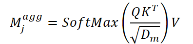
This approach makes it possible to accurately extract only the relevant details from the target feature, even when the motion occurs in complex or nonlinear regions.
The final combination of movements is performed using the following formula:

In other words, the attention map amplifies the useful components, after which the original neighboring feature is added to them to maintain stability. A similar procedure is applied to the backward motion features, resulting in symmetrically enriched forward and backward motion features.
In the final stage, all the features obtained are fed into ConvGRU, which updates the optical flow based on all the collected temporal information. This approach provides a more consistent and detailed motion estimate, especially in dynamic and visually complex scenes.
The author's visualization of the BAT framework is shown below.


Implementation in MQL5
Now that we have thoroughly examined the theoretical foundation of the BAT framework and evaluated its advantages, it is time to move on to the practical aspects of the project. Currently, we are interested not only in the concept, but also in its actual implementation using MQL5. It is here that ideas begin to take shape, and abstract designs are transformed into working mechanisms ready to interact with live market data streams.
There is a lot of work ahead. The BAT framework's algorithm is multi-layered, and — much like a thoughtful trader who prefers not to open dozens of positions at once — we will not dive into all the details right away. It makes more sense to proceed step by step, breaking the entire process down into neat functional blocks. This approach creates a robust structure and reduces the risk of errors, which ultimately improves the quality of implementation and facilitates subsequent optimization.
We will start with the very basics — input data representation. In our case, we assume that the model will receive data directly from the terminal. In other words, all stages of data preparation — including normalization and conversion to a format resembling the structure of optical flow — remain the responsibility of the framework's internal logic. This approach preserves flexibility and makes the model self-contained, eliminating the need for unnecessary external manipulation.
To adapt market data to the concept of temporal flow used by the framework's authors, we need to construct an event structure. Each step of the model must account for the changes that occur between two consecutive points in time. Therefore, the key operation at this stage is simple yet fundamental: we calculate the difference between two adjacent states and, at the same time, save the current state so that we can use it in the next cycle. In this way, we create an analogue of optical displacement, allowing the model to perceive the market not as a set of static quantities, but as a dynamic process with its own speed, direction, and temporal texture.
This step paves the way for the entire subsequent architecture. It sets the rhythm, defines the structure, and ensures the temporal consistency of the data — without which the BAT framework cannot reach its full potential.
To set up basic data processing and generate an initial motion vector between two consecutive states, let’s start with a simple but extremely important step — creating a small compute kernel in the OpenCL program. It will record the changes between the current and previous states of the data array being analyzed, thereby creating an analogue of elementary optical flow.
There is no complicated logic here — and that is what makes it so powerful. The kernel's task is strictly functional: take the current value, compare it to the previous one, calculate the difference, and save the updated state for the next iteration. And all of this is done in the streaming style characteristic of OpenCL.
__kernel void CalcFlow(__global const float* value,
                       __global float* prev_value,
                       __global float* flow
                      )
  {
   const size_t id = get_global_id(0);
   const size_t total = get_global_size(0);
//---
   const float v = IsNaNOrInf(value[id], 0);
   const float p = IsNaNOrInf(prev_value[id], 0);
   flow[id] = IsNaNOrInf(v - p, 0);
   prev_value[id] = v;
  }
Despite its simplicity, this kernel plays an important role. It creates an initial dynamic data structure, which can then be used as a basis for further transformations. This step is fully in line with the BAT concept, which focuses primarily on extracting temporal structure from a data stream.
Next, we turn to the main program and build the infrastructure that connects the computational flow of the OpenCL program with the neural network's logic. This is where a new class — CNeuronCreateFlow — comes into play. It serves as the interface layer that manages states, invokes the compute kernel, and organizes the data flow — but its functions are not limited to these.
The main idea behind the block is as simple as a good market strategy — do not waste resources on unnecessary computations, and use information only where it is actually updated. The difference between two fixed historical states remains constant. This means that it makes no sense to recalculate it at every iteration of the model.
Therefore, the CNeuronCreateFlow component focuses on something else: it calculates only the changes between the latest (current) state and the immediately preceding state. This logic fully reflects both the design philosophy of BAT and the nature of the market data stream, which continuously shifts over time but retains only the latest change.
After obtaining the next difference vector, the data is pushed onto the stack. In this way, we generate a sequence of temporal shifts — the market’s microdynamics — which will subsequently be transformed into more complex structures: temporal groups, correlation maps, aggregated features, and other elements of the BAT algorithm.
This stack serves as the equivalent of a temporal grid in optical flow problems. Each new slice captures short-term changes in price or features. And the model's architecture extracts from these shifts the dynamics needed to analyze deeper patterns.
In fact, CNeuronCreateFlow is a small but crucial component. It ensures a continuous supply of correct temporal data to the model, eliminates redundant calculations, and lays the groundwork for the next stages.
class CNeuronCreateFlow :  public CNeuronSpikePatchStak
  {
protected:
   CNeuronBaseOCL*   cState;
   //---
   virtual bool      CalcFlow(CNeuronBaseOCL *NeuronOCL);
   virtual bool      feedForward(CNeuronBaseOCL *NeuronOCL) override;
   virtual bool      updateInputWeights(CNeuronBaseOCL *NeuronOCL) override;
   virtual bool      calcInputGradients(CNeuronBaseOCL *NeuronOCL) override;

public:
                     CNeuronCreateFlow(void) {};
                    ~CNeuronCreateFlow(void) {};
   //---
   virtual bool      Init(uint numOutputs, uint myIndex, COpenCLMy *open_cl,
                          uint stack_size, uint dimension,
                          uint patch_dimension, uint variables,
                          ENUM_OPTIMIZATION optimization_type, uint batch);
   //---
   virtual int       Type(void)   override const   {  return defNeuronCreateFlow;   }
   //--- methods for working with files
   virtual bool      Load(int const file_handle) override;
   //---
   virtual void      SetOpenCL(COpenCLMy *obj)   override;
   //---
   virtual bool      Clear(void) override;
  };
The class structure is simple and elegant. Inside CNeuronCreateFlow, we declare just one key component — cState. It serves a dual purpose: on the one hand, it stores the current difference between the latest and previous states, and on the other, it contains a tensor that describes the latest state of the system. Thus, cState serves both as a repository for current changes and as the basis for the next processing step.
All other functionality related to organizing and managing the flow dynamics stack is inherited from the parent class, CNeuronSpikePatchStak. This solution highlights the modularity of the architecture. The main class is responsible for storing and sequentially updating temporal information, managing the stack, and preparing data for subsequent framework modules.
It is worth paying special attention to one important point. The parent class does not simply store a raw vector of changes between states on the stack; instead, it generates a trainable embedding that encodes these changes into a compact and informative representation. This approach has several advantages: the embedding reduces the size of the data, makes it more suitable for subsequent processing, and allows the model to identify precisely those aspects of the dynamics that are most important for accurate optical flow estimation.
The initialization of a new object builds on the solid foundation of the parent class and carefully extends its functionality, creating a workspace for storing and processing flow dynamics.
bool CNeuronCreateFlow::Init(uint numOutputs, uint myIndex, COpenCLMy *open_cl,
                             uint stack_size, uint dimension,
                             uint patch_dimension, uint variables,
                             ENUM_OPTIMIZATION optimization_type, uint batch)
  {
   if(!CNeuronSpikePatchStak::Init(numOutputs, myIndex, open_cl, stack_size,
                                   dimension, patch_dimension, variables, optimization_type, batch))
      return false;
First, the parent class is initialized. This is a crucial step. This is where the basic structures for the dynamics stack are created, internal buffers are allocated, and training parameters are set. If initialization of the parent class fails, the method immediately returns false, protecting the system from incorrect operation.
Next, the internal component cState is initialized. It is allocated storage for the current difference between states and a tensor describing the latest state. The parameters passed to this stage take into account the dimensionality of the data being analyzed, ensuring proper alignment with the main model.
   if(!cState.Init(0, 0, OpenCL, dimension * variables, optimization, iBatch))
      return false;
The final step is to call the Clear method, which clears all internal buffers and ensures that the object starts from a clean state.
   if(!Clear())
      return false;
//---
   return true;
  }
Only after these steps have been successfully completed does the method return true, indicating that the object is ready for use.
As a result, we obtain a fully prepared component capable of accurately capturing changes between successive states and passing them to the model's dynamics stack, ensuring that embeddings are formed correctly.
The forward pass algorithm has a concise, linear implementation. The feedForward method first calls CalcFlow, which, as we have already discussed, calculates the difference between the current and previous states, updating the internal cState component. If the flow calculation fails, the method immediately returns false, preventing incorrect data from propagating further through the model.
bool CNeuronCreateFlow::feedForward(CNeuronBaseOCL *NeuronOCL)
  {
   if(!CalcFlow(NeuronOCL))
      return false;
//---
   return CNeuronSpikePatchStak::feedForward(cState.AsObject());
  }
The object then passes the result to the method of the same name in the parent class. It is the parent class that is responsible for organizing the temporal dynamics stack, updating embeddings, and integrating features into the overall model architecture.
Thus, the feedForward method combines a simple, linear difference calculation with the powerful functionality of its parent. The forward pass remains lightweight and efficient, while all calculated changes are immediately and accurately incorporated into the model's dynamics stack, ready for subsequent processing steps.
It is important to emphasize one key point here — we deliberately did not create a separate kernel for the backward pass. At first glance, this might seem like a limitation, but in practice it poses no problem if the object is used as the model's first layer, directly processing input data that does not depend on previous layers.
However, when this block is used as an internal layer of the model, the error gradient must be propagated correctly. This is necessary so that the preceding neural layers can be trained correctly, using information about how changes in their outputs affect the final result.
Our kernel calculates the difference between the latest and previous states. This offers an important advantage: the gradient with respect to the current state can be passed directly to the previous values without any additional operations. In this way, we preserve the linearity and simplicity of the calculations while ensuring that errors are propagated correctly.
The calcInputGradients method implements this mechanism. First, the pointer to the source data object is checked for validity.
bool CNeuronCreateFlow::calcInputGradients(CNeuronBaseOCL *NeuronOCL)
  {
   if(!NeuronOCL)
      return false;
//---
   if(!CNeuronSpikePatchStak::calcInputGradients(cState.AsObject()))
      return false;
   if(!DeActivation(NeuronOCL.getOutput(), NeuronOCL.getGradient(),
                    cState.getGradient(), NeuronOCL.Activation()))
      return false;
//---
   return true;
  }
Next, the method of the same name in the parent class is called to work with the cState embedding stack. DeActivation is then applied to propagate the gradients correctly to the source data object, taking its activation function into account.
In this way, we achieve two goals at once: we preserve the simplicity of the architecture and ensure full differentiability. Gradients are correctly propagated to the source data object, allowing the previous layers of the model to be trained without the need to create a separate backward pass kernel.
We have done a lot of work today and deserve a short break. Let's give ourselves a moment to let this information sink in, and in the next article — with renewed energy and a fresh perspective — we will continue our exploration of the practical implementation of the BAT framework's algorithms, uncovering its capabilities and features step by step.
Conclusion
The BAT framework shows great potential for analyzing financial market dynamics by combining accuracy with adaptability in processing time-series data. Its architecture makes it possible to transform sequential changes in market states into structured representations, ensuring dense and informative encoding of the dynamics. The use of bidirectional adaptive temporal correlation and aggregation mechanisms enables the model to identify both short-term and long-term movement patterns.
Overall, BAT offers a unique balance between flexibility and computational efficiency, transforming complex time-series data into accurate and structured signals for decision-making in financial markets.
Links
- BAT: Learning Event-Based Optical Flow with Bidirectional Adaptive Temporal Correlation
- Other articles in this series
Software used in this article
| # | Name | Type | Description |
|---|---|---|---|
| 1 | Study.mq5 | Expert Advisor | Expert Advisor for offline model training |
| 2 | StudyOnline.mq5 | Expert Advisor | Expert Advisor for online model training |
| 3 | Test.mq5 | Expert Advisor | Expert Advisor for model testing |
| 4 | Trajectory.mqh | Class library | Structure describing the system state and model architectures |
| 5 | NeuroNet.mqh | Class library | Class library for building a neural network |
| 6 | NeuroNet.cl | Library | OpenCL program code library |
Translated from Russian by MetaQuotes Ltd.
Original article: https://www.mql5.com/ru/articles/20506
Warning: All rights to these materials are reserved by MetaQuotes Ltd. Copying or reprinting of these materials in whole or in part is prohibited.
This article was written by a user of the site and reflects their personal views. MetaQuotes Ltd is not responsible for the accuracy of the information presented, nor for any consequences resulting from the use of the solutions, strategies or recommendations described.