Neural Networks in Trading: Effective Feature Extraction for Accurate Classification (Final Part)

Introduction

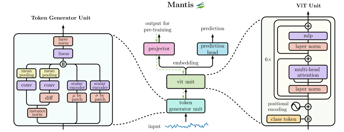
We have reached the final phase of our introduction to the Mantis framework. First, we examined its theoretical foundation in detail: how the model processes multichannel time series, why difference signals are needed, and how local tokens are formed. We then delved deeper into the architecture to see how the patches are structured and how the model learns to extract stable patterns from market noise. Now is the time to bring it all together.

The Mantis framework is structured as a sequence of independent but logically related modules. Each of them performs a specialized task — from the initial processing of input data to token formation and information aggregation. The underlying principle is this: minimal bias while extracting as many patterns as possible from the data itself.

It all starts with raw market features entering the model. Instead of treating them as a single matrix, the model separates each data type into a separate channel. For each one, an additional channel of first differences is created, allowing the model to explicitly capture short-term dynamics. Such difference channels increase the model's sensitivity to changes in the direction of price movement. For example, a sudden acceleration in the difference channel may indicate the start of a impulse move long before indicators detect it.

Each of these channels is fed to the convolutional blocks. This is where the initial analysis begins. Convolutions extract local features by learning to distinguish stable micro-patterns. Each channel produces 256 features representing its local behavior.

After convolution, the next stage begins: the data is divided into 32 non-overlapping patches. Each of them covers a specific segment of the time series. For each one, channel-wise averaging (mean-pooling) is performed. This gives us 32 tokens, each with 256 features. This is an important point. Patches are localized segments of market behavior — essentially condensed mini-charts. They capture phases ranging from impulse / impulse moves and consolidations to pullbacks and divergences. This type of partitioning makes the model's behavior more stable and adaptive. It begins to see the market not as a stream of numbers but as a series of recognizable scenarios.

At this stage, for each input data channel, a token is taken from the original stream and the difference stream. These tokens are scaled to a common range, normalized, and combined. A summary token is then produced by a linear projection layer, reflecting the behavior of this channel over the specified segment. Such a token contains the state, the rate of change, and the strength. Everything that allows a trader to intuitively gauge market sentiment.

Next, the entire sequence of tokens is fed into attention blocks. This is the most critical level, where patches begin to communicate with one another. The model assesses which segments of the past are important for the current state. Perhaps a signal that emerged 20 bars ago is now becoming critical for assessing a reversal. This ability to see connections between distant segments makes the model particularly useful for analyzing complex market structures.

Behind all of this lies a simple yet powerful idea: to maintain local precision without losing sight of the global context. In trading, this is critical. For example, a sequence of small candles during a lull may contain little or no information. But if they appear after a sharp spike in volume — especially at a significant level — the context changes completely. Mantis takes this into account automatically.

The Mantis framework is more than just an architecture. It is a flexible tool capable of adapting to various types of trading strategies.

The author's visualization of the Mantis framework is shown below.

Model Architecture

In previous articles, we have already built the main components of the Mantis framework, and we have now reached a key stage: designing the architecture of a trainable model capable of making trading decisions in real time. Just like an experienced trader who monitors price behavior, volumes, candlestick patterns, and overall market sentiment — and only then, taking the context into account, makes a decision to enter a trade — our model must learn to perceive market dynamics not as a stream of numbers, but as a set of interconnected processes. We aim to replicate a behavioral model that can distinguish market patterns, sense shifts in market phases, and adapt to new scenarios. It is precisely in this context that the logic of the entire Mantis framework is built.

It should be emphasized that the Mantis framework was originally developed as a time-series classifier. Its architecture is designed for segmenting and identifying hidden patterns in complex sequences. This approach has proven particularly effective in the financial context, where price movements are often hidden beneath layers of market noise. Through multi-level processing — including convolutions, local patch formation, and channel aggregation — the model learns to see structure in market data rather than random fluctuations. Mantis makes it possible not only to capture signals but also to identify market regimes.

However, in the context of our current task, Mantis no longer functions as a standalone classifier, but rather as the foundation — the foundation of the trading agent’s perceptual layer. We use the Mantis architecture to build an embedding — a compact yet information-rich representation of the market situation — which is then fed into the control component of the model. In this way, the classifier becomes the agent's eyes, giving it the ability to see the behavioral fabric of the market.

It is precisely this embedding that is passed on to the next part of the architecture, which is based on the Actor–Director–Critic principle. This approach allows responsibilities to be divided among modules and ensures the stability of the agent’s behavior. The Actor receives an embedding and forms a trading decision. The Director acts as a structural filter and behavioral corrector, classifying the actions proposed by the Actor as either valid or erroneous and providing strong feedback signals. Its purpose is to filter out clearly unreasonable or unstable decisions, especially in zones of market turbulence. The Critic completes the cycle by assessing the strategic soundness of actions based on the current state and the history of interactions. It acts as an internal advisor: even if an action is possible, is it really worth the risk in the current context?

The architecture of all model components is defined using the CreateDescriptions method, in which the layers of each module are configured sequentially. A flexible parameter system makes it possible to scale the architecture, adapt it to various market instruments, and add or disable experimental elements without having to rewrite the core logic.

bool CreateDescriptions(CArrayObj *&encoder,
                        CArrayObj *&actor,
                        CArrayObj *&director,
                        CArrayObj *&critic
                       )
  {
//---
   CLayerDescription *descr;
//---
   if(!encoder)
     {
      encoder = new CArrayObj();
      if(!encoder)
         return false;
     }
   if(!actor)
     {
      actor = new CArrayObj();
      if(!actor)
         return false;
     }
   if(!director)
     {
      director = new CArrayObj();
      if(!director)
         return false;
     }
   if(!critic)
     {
      critic = new CArrayObj();
      if(!critic)
         return false;
     }

Through the method parameters, we receive pointers to four dynamic arrays, each intended to store the architectural descriptions of the corresponding model components: the Encoder, the Actor, the Director, and the Critic. These arrays act as containers into which objects describing the structure of the neural network blocks are added one by one.

Inside the method body, the first step is to validate the received pointers. If any of them is uninitialized or points to an invalid memory location, a new instance of the corresponding object is automatically created. This approach eliminates the need to manually prepare arrays in advance, thereby increasing the code's modularity and its suitability for scalable solutions.

Next, we move directly to the description of the model architectures. It is logical to present the Encoder first in this chain — the key module through which the model begins to perceive the market. This is where the process of transforming raw time series into a meaningful representation of the market state begins.

At the first stage, we use a fully connected layer, which in this case does not perform a computational function but solely an interface one. Its role is to provide a convenient buffer interface for loading the input data into the model.

//--- Encoder
   encoder.Clear();
//--- Input layer
   if(!(descr = new CLayerDescription()))
      return false;
   descr.type = defNeuronBaseOCL;
   int prev_count = descr.count = (HistoryBars * BarDescr);
   descr.activation = None;
   descr.optimization = ADAM;
   if(!encoder.Add(descr))
     {
      delete descr;
      return false;
     }

Disparate input data with different scales are passed to the batch normalization block. Here, all values are brought to a comparable scale, and differences in scale are reduced, which is especially critical when working with multidimensional financial time series. Normalization allows the model to perceive the data not as a random set of numbers, but as a logically coherent stream of information.

//--- layer 1
   if(!(descr = new CLayerDescription()))
      return false;
   descr.type = defNeuronBatchNormWithNoise;
   descr.count = prev_count;
   descr.batch = 1e4;
   descr.activation = None;
   descr.optimization = ADAM;
   if(!encoder.Add(descr))
     {
      delete descr;
      return false;
     }

For mild data augmentation during training, we use a batch normalization layer with controlled noise added, which helps make the model more robust to market noise and helps prevent it from overfitting to insignificant fluctuations. This approach helps the system interpret market information more flexibly while maintaining a balance between adaptation and stability.

The next important step is to create first-difference channels. This layer generates difference features — changes in values between adjacent time points — which help the model capture the dynamics and direction of market movement. In trading, it is precisely these changes that often provide the key to understanding trend reversals or trend continuation, since a rise or fall in price at a given moment can sometimes be more important than absolute values. Creating difference channels significantly enhances the informational content of the source data, increasing the model's sensitivity to local trends and rapid fluctuations.

//--- layer 2
   if(!(descr = new CLayerDescription()))
      return false;
   descr.type = defNeuronConcatDiff;
   prev_count = descr.count = HistoryBars;
   descr.layers = BarDescr;
   descr.step = 1;
   descr.batch = 1e4;
   descr.optimization = ADAM;
   descr.activation = None;
   if(!encoder.Add(descr))
     {
      delete descr;
      return false;
     }

After the first-difference channels have been formed, temporal encoding harmonics are added to the expanded dataset. This step is extremely important for enabling the model to understand the context of temporal dependencies and the cyclical nature of market processes. Harmonics are a kind of temporal beacon that allows the model to recognize not only a specific point in time, but also recurring patterns, seasonal fluctuations, and various time scales. Temporal encoding via harmonics provides the model with a deep understanding of the temporal structure.

//--- layer 3
   if(!(descr = new CLayerDescription()))
      return false;
   descr.type = defMamba4CastEmbeding;
   prev_count = descr.count = HistoryBars;
   descr.window = 2 * BarDescr;
   int prev_out = descr.window_out = NSkills;
     {
      int temp[] = {PeriodSeconds(PERIOD_H1), PeriodSeconds(PERIOD_D1)};
      if(ArrayCopy(descr.windows, temp) < (int)temp.Size())
         return false;
     }
   descr.batch = 1e4;
   descr.optimization = ADAM;
   descr.activation = None;
   if(!encoder.Add(descr))
     {
      delete descr;
      return false;
     }

To effectively account for cross-channel relationships and interdependencies in the data, we use a convolution block with different window sizes. This multi-window approach allows the model to simultaneously capture both local, short-term patterns and longer-term trends that appear in the dynamics across multiple channels at once.

//--- layer 5
   if(!(descr = new CLayerDescription()))
      return false;
   descr.type = defNeuronBatchNormOCL;
   descr.count = prev_count * prev_out;
   descr.batch = 1e4;
   descr.activation = None;
   descr.optimization = ADAM;
   if(!encoder.Add(descr))
     {
      delete descr;
      return false;
     }

The final stage of data preparation is the patching layer. This layer divides the processed multichannel tensor into separate, non-overlapping patches — essentially fragments of the time series, each of which contains grouped information about local market conditions.

This partitioning allows the model to focus on individual data segments, reducing computational complexity and making it easier to identify local patterns. Additional aggregation is performed within each patch, ensuring a compact yet informative representation.

As a result, each patch becomes a separate token carrying a compressed and structured description of the market situation over a limited time interval. This significantly improves the model's ability to capture local patterns and provides a solid foundation for subsequent processing and decision-making stages.

//--- layer 6
   if(!(descr = new CLayerDescription()))
      return false;
   descr.type = defNeuronMantisPatching;
   descr.count = prev_count;
   descr.layers = prev_out;
   descr.window = EmbeddingSize;
   descr.window_out = NSkills;
   descr.step = Segments;
   descr.batch = 1e4;
   descr.optimization = ADAM;
   descr.activation = None;
   if(!encoder.Add(descr))
     {
      delete descr;
      return false;
     }
   prev_count = descr.step;
   prev_out = descr.layers;

The attention block in our Encoder is implemented as a single object: CNeuronMantisAttentionUnit. This component plays a key role in capturing important relationships between patches and channels. In the object's parameters, we specify the number of internal cross-attention modules, which allows us to flexibly adjust the depth and breadth of information analysis.

Each cross-attention module focuses on identifying the most significant elements in the data stream, relating them to a learnable class token. This architecture provides effective noise filtering and helps the model focus specifically on the signals that actually influence trading decisions.

//--- layer 7
   if(!(descr = new CLayerDescription()))
      return false;
   descr.type = defNeuronMantisAttentionUnit;
   descr.step = 4;
   descr.count = prev_count;
     {
      int temp[] = {EmbeddingSize, EmbeddingSize};
      if(ArrayCopy(descr.windows, temp) < (int)temp.Size())
         return false;
     }
   descr.layers = 3;
   descr.window_out = NSkills;
   descr.window = prev_out;
   descr.batch = 1e4;
   descr.optimization = ADAM;
   descr.activation = None;
   if(!encoder.Add(descr))
     {
      delete descr;
      return false;
     }

At the output of the cross-attention module, a token is generated — a compact and informative representation of the analyzed state of the environment. In the context of our task, accurate classification of states is not a priority. It is more important for us to obtain sufficiently clear and distinct latent representations that will enable the Actor to make well-considered and informed trading decisions.

That is precisely why we deliberately chose not to overcomplicate the architecture of the Encoder. This approach maintains a balance between the depth of the model's perception and its computational efficiency, allowing it to adapt flexibly to real-world market conditions without compromising the quality of the decisions made.

Next, we move on to a description of the architecture of the Actor. As in the case of the Encoder, the input stage uses a combination of a fully connected layer and a batch normalization block. This pair serves as an interface for receiving and initially standardizing the input data. However, in this case, the main information channel carries different information: data on the current state of the trading account, including the balance, open positions, drawdown level, and other metrics that reflect the internal operating context of the trading agent.

//---
   CLayerDescription *latent = encoder.At(7);
//--- Actor
   actor.Clear();
//--- Input layer
   if(!(descr = new CLayerDescription()))
      return false;
   descr.type = defNeuronBaseOCL;
   descr.count = AccountDescr;
   descr.activation = None;
   descr.optimization = ADAM;
   if(!actor.Add(descr))
     {
      delete descr;
      return false;
     }
//--- layer 1
   if(!(descr = new CLayerDescription()))
      return false;
   descr.type = defNeuronBatchNormOCL;
   descr.count = AccountDescr;
   descr.batch = 1e4;
   descr.activation = None;
   descr.optimization = ADAM;
   if(!actor.Add(descr))
     {
      delete descr;
      return false;
     }

In parallel, via an auxiliary channel, a latent representation of the market environment formed by the Encoder is fed into the model. By combining these two data streams — internal state and external context — the Actor is able to make decisions that already incorporate an element of strategic thinking and risk management. The model is trained to take into account not only the current market situation, but also its own resources, its risk tolerance, and the dynamics of its current position. This approach makes the Agent's behavior deliberate and robust, even amid heightened market turbulence.

Data from two information streams — market context and the state of the trading account — are consolidated in the concatenation layer. This object performs a simple but important function: it combines the embedding vector received from the Encoder with the internal characteristics of the trading account into a single representation. In this way, the model obtains a complete picture of what is happening.

//--- layer 2
   if(!(descr = new CLayerDescription()))
      return false;
   descr.type = defNeuronConcatenate;
   descr.count = LatentCount;
   descr.window = AccountDescr;        // Inputs window
   descr.step = latent.windows[0];     // Cross window
   descr.batch = 1e4;
   descr.activation = TANH;
   descr.optimization = ADAM;
   if(!actor.Add(descr))
     {
      delete descr;
      return false;
     }

After the data is combined, deep feature processing begins, implemented through a sequence of three fully connected layers. The first layer is responsible for extracting and generalizing key features. The second layer strengthens significant dependencies between parameters, revealing potential patterns. In the third layer, a trading action is formed. This sequential transformation enables the model not simply to respond to signals, but to make well-considered and strategically sound decisions.

//--- layer 3
   if(!(descr = new CLayerDescription()))
      return false;
   descr.type = defNeuronBaseOCL;
   descr.count = LatentCount;
   descr.batch = 1e4;
   descr.activation = TANH;
   descr.optimization = ADAM;
   if(!actor.Add(descr))
     {
      delete descr;
      return false;
     }
//--- layer 4
   if(!(descr = new CLayerDescription()))
      return false;
   descr.type = defNeuronBaseOCL;
   descr.count = LatentCount;
   descr.activation = SoftPlus;
   descr.batch = 1e4;
   descr.optimization = ADAM;
   if(!actor.Add(descr))
     {
      delete descr;
      return false;
     }
//--- layer 5
   if(!(descr = new CLayerDescription()))
      return false;
   descr.type = defNeuronBaseOCL;
   prev_count = descr.count = NActions;
   descr.activation = SIGMOID;
   descr.batch = 1e4;
   descr.optimization = ADAM;
   if(!actor.Add(descr))
     {
      delete descr;
      return false;
     }

The architecture of the Director and Critic models almost completely mirrors the structure of the Actor model. The main difference lies in the dimensionality of the input data. The action tensor of the Agent is fed to these models via the main channel, and at the output an evaluation of these actions is formed — a classification evaluation by the Director and a strategic evaluation by the Critic. Since the internal logic of these models is similar, we will not overload the article by describing them again. For a more detailed examination, readers may refer to the code accompanying this article, which provides a complete description of the architecture of all the system’s trainable components.

Contrastive Learning

After building the architectures of the models, we move on to the next important stage — training. As discussed in detail in the theoretical section, one of the key features of the Mantis framework is self-supervised contrastive learning. This mechanism allows the model to generate informative and clearly distinguishable tokens that describe the state of the environment in a compact yet expressive form. Just as an experienced trader can distinguish a consolidation phase from a impulse move at a glance, our model must learn to identify characteristic market conditions and represent them in a condensed form for subsequent use by other components of the system.

In this case, contrastive learning serves as the foundation for developing market intuition in the model. Without strict supervision, but with a clear understanding of the differences between pairs of states, the Encoder learns to construct representations that will help it distinguish as effectively as possible between similar but fundamentally different market scenarios.

The implementation of the corresponding algorithm is provided in the Expert Advisor (EA) "…\MQL5\Experts\Mantis\StudyContrast.mq5". The EA manages the process of forming pairs of positive and negative examples, runs a training iteration, collects statistics, and saves the trained parameters.

It is worth noting one important — and, without exaggeration, conceptual — difference between our implementation of contrastive learning and traditional approaches. We have deliberately chosen to omit the time-consuming step of forming a training dataset at this stage of training. Instead, by leveraging the full power and flexibility of the MetaTrader 5 platform, we implemented dynamic generation of training data during the training process.

All the user needs to do is specify the start and end dates of the training period in the EA settings. All necessary market data is automatically requested and retrieved from the terminal in real time. This approach not only simplifies the procedure but also provides much broader possibilities when training the model.

//+------------------------------------------------------------------+
//| Input parameters                                                 |
//+------------------------------------------------------------------+
input datetime             Start          = D'2020.01.01';
input datetime             End            = D'2025.01.01';
input int                  Iterations     = 100000;
input int                  Batch          = 50;
input group                "---- Indicators ----"
input ENUM_TIMEFRAMES      TimeFrame   =  PERIOD_M1;
//---
input group                "---- RSI ----"
input int                  RSIPeriod   =  14;            //Period
input ENUM_APPLIED_PRICE   RSIPrice    =  PRICE_CLOSE;   //Applied price
//---
input group                "---- CCI ----"
input int                  CCIPeriod   =  14;            //Period
input ENUM_APPLIED_PRICE   CCIPrice    =  PRICE_TYPICAL; //Applied price
//---
input group                "---- ATR ----"
input int                  ATRPeriod   =  14;            //Period
//---
input group                "---- MACD ----"
input int                  FastPeriod  =  12;            //Fast
input int                  SlowPeriod  =  26;            //Slow
input int                  SignalPeriod =  9;            //Signal
input ENUM_APPLIED_PRICE   MACDPrice   =  PRICE_CLOSE;   //Applied price

Next, I’d like to take a closer look at how this process is implemented in the Train method. This method starts the entire contrastive learning cycle and contains the logic for data preparation, buffer management, and forward and backward passes through the network.

The process begins by defining the boundaries of the historical data. The iBarShift function is used to determine the offset from the current bar to the start and end of training.

void Train(void)
  {
   int start = iBarShift(Symb.Name(), TimeFrame, Start);
   int end = iBarShift(Symb.Name(), TimeFrame, End);
   int bars = CopyRates(Symb.Name(), TimeFrame, 0, start, Rates);

Next, buffers for all indicators are allocated to accommodate the length of the history being loaded.

if(!RSI.BufferResize(bars) || !CCI.BufferResize(bars) ||
   !ATR.BufferResize(bars) || !MACD.BufferResize(bars))
  {
   PrintFormat("%s -> %d", __FUNCTION__, __LINE__);
   ExpertRemove();
   return;
  }

The next stage is data loading. To do this, a loop is implemented that sequentially calls the Refresh methods of all indicators and checks the number of calculated values. The loop will end either after the data has been loaded successfully or after 100 attempts.

int count = -1;
bool load = false;
do
  {
   RSI.Refresh();
   CCI.Refresh();
   ATR.Refresh();
   MACD.Refresh();
   count++;
   load = (RSI.BarsCalculated() >= bars &&
           CCI.BarsCalculated() >= bars &&
           ATR.BarsCalculated() >= bars &&
           MACD.BarsCalculated() >= bars
          );
   Sleep(100);
   count++;
  }
while(!load && count < 100);
if(!load)
  {
   PrintFormat("%s -> %d The training data has not been loaded",
                                        __FUNCTION__, __LINE__);
   ExpertRemove();
   return;
  }

At the end of the data preparation process, we set the required indexing direction for the quote array (ArraySetAsSeries) and declare the necessary local variables.

   if(!ArraySetAsSeries(Rates, true))
     {
      PrintFormat("%s -> %d", __FUNCTION__, __LINE__);
      ExpertRemove();
      return;
     }
   bars -= end + HistoryBars;
   if(bars < 0)
     {
      PrintFormat("%s -> %d", __FUNCTION__, __LINE__);
      ExpertRemove();
      return;
     }
//---
   vector<float> result, target, neg_target;
   bool Stop = false;

The main training loop now begins. In each iteration, a position — the bar index from which the reference state will be formed — is randomly selected from the overall range.

   uint ticks = GetTickCount();
//---
   for(int iter = 0; (iter < Iterations && !IsStopped() && !Stop); iter += Batch)
     {
      int posit = (int)((MathRand() * MathRand() / MathPow(32767, 2)) * bars);
      if(!CreateBuffers(posit + end, GetPointer(bState), GetPointer(bTime)))
        {
         PrintFormat("%s -> %d", __FUNCTION__, __LINE__);
         ExpertRemove();
         return;
        }

For this state, source data buffers are created and a forward pass through the Encoder is performed.

//--- Feed Forward
if(!cEncoder.feedForward((CBufferFloat*)GetPointer(bState), 1, false,
                                   (CBufferFloat*)GetPointer(bTime)))
  {
   PrintFormat("%s -> %d", __FUNCTION__, __LINE__);
   Stop = true;
   break;
  }
cEncoder.getResults(Result);

We save the result of the forward pass as a reference — a kind of sample market state that the model will aim to match. Next, and importantly, a forward pass through the Encoder is performed again using exactly the same input data. But there is a subtlety here. The batch normalization layer with added noise built into our architecture acts as a mild form of data augmentation. This means that during the repeated pass, the model no longer simply repeats the previous result, but produces a slightly altered, noisy output.

It is precisely this property that we use to form a positive pair. The backward pass is performed using the previously saved reference as the target. In this way, we train the model to ignore random noise and focus on meaningful, stable contextual features. Simply put, the model learns to see through the noise and maintain a stable view of key market characteristics.

//--- Positive
if(!cEncoder.feedForward((CBufferFloat*)GetPointer(bState), 1, false,
                                 (CBufferFloat*)GetPointer(bTime)) ||
   !cEncoder.backProp(Result, (CBufferFloat*)NULL))
  {
   PrintFormat("%s -> %d", __FUNCTION__, __LINE__);
   Stop = true;
   break;
  }

Next comes what is perhaps the most interesting part — forming negative pairs. The number of negative pairs is specified in the EA parameters by the Batch variable. To generate the required number of negative pairs, we create a nested loop, having first moved the reference token into a vector.

//--- Negative
if(!Result.GetData(target))
  {
   PrintFormat("%s -> %d", __FUNCTION__, __LINE__);
   Stop = true;
   break;
  }
for(int b = 0; b < Batch; b++)
  {
   int negot = (int)((MathRand() * MathRand() / MathPow(32767, 2)) * bars);
   int count = 0;
   while(negot == posit)
     {
      negot = (int)((MathRand() * MathRand() / MathPow(32767, 2)) * bars);
      count++;
      if(count > 100)
        {
         PrintFormat("%s -> %d", __FUNCTION__, __LINE__);
         Stop = true;
         break;
        }
     }
   if(Stop)
            break;

In the body of the nested loop, we randomly select another state from the training range — one that is different from the previously used reference state. It is worth emphasizing an important point here: we accept any state, as long as it does not match the reference state. In theory, it is even possible for the ranges to overlap.

This is exactly what makes the training process more dynamic and realistic. The model learns to identify differences in very similar states. If the ranges overlap, the model's task is to highlight precisely those nuances that distinguish one state from another. In real-world market conditions, it is precisely these subtle differences that often determine the success of a trading decision.

Thus, our contrastive training compels the Encoder not merely to recognize states, but to extract key features, creating informative and distinguishable tokens needed for the subsequent operation of the Actor.

For the selected state, we generate the source data buffers and perform a forward pass through the Encoder.

if(!CreateBuffers(negot + end, GetPointer(bState), GetPointer(bTime)))
  {
   PrintFormat("%s -> %d", __FUNCTION__, __LINE__);
   ExpertRemove();
   return;
  }
//--- Feed Forward
if(!cEncoder.feedForward((CBufferFloat*)GetPointer(bState), 1, false,
                                   (CBufferFloat*)GetPointer(bTime)))
  {
   PrintFormat("%s -> %d", __FUNCTION__, __LINE__);
   Stop = true;
   break;
  }

Next comes the stage of forming the training targets for the negative training example. To do this, we calculate the difference between the token obtained at the current step and the reference representation that we saved earlier. This is the key point: we push the current token away from the reference, creating a target value for the negative example.

To amplify this effect, we double the distance between the reference state and the current state, thereby increasing the repulsive force. As a result, states that are close to the reference state are repelled only slightly, while those that differ significantly are repelled with much greater intensity. This helps expand the free space around the reference representation, making the tokens more distinguishable and more robust against noise.

This mechanism introduces a dynamic element into the learning process that ensures a clear separation of latent spaces. The model does not simply learn to recognize states; it learns to create a safety zone around the reference state, keeping other, different states at a noticeable distance. This significantly improves the quality and reliability of subsequent decision-making.

cEncoder.getResults(result);
neg_target = result * 2 - target;
neg_target = neg_target - neg_target.Max();
if(!neg_target.Activation(neg_target, AF_SOFTMAX) ||
   !Result.AssignArray(neg_target))
  {
   PrintFormat("%s -> %d", __FUNCTION__, __LINE__);
   Stop = true;
   break;
  }

We have one last, but no less important, step left: to perform a backward pass through the Encoder using the generated negative target. It is this stage that allows the model's parameters to be optimized, adjusting it so that it effectively pushes distinct states away from one another in the latent space.

if(!cEncoder.backProp(Result, (CBufferFloat*)NULL))
  {
   PrintFormat("%s -> %d", __FUNCTION__, __LINE__);
   Stop = true;
   break;
  }

Now that all training operations for this step have been successfully completed, the system keeps the user informed — the process status is updated. We provide updates on current progress by showing the completion percentage and the model's error metrics. This transparent approach not only builds trust in the algorithm's performance but also helps to quickly monitor the effectiveness of the training.

After that, we move on to the next iteration of the training loop, where the entire process described above is repeated again with new data. This cycle ensures thorough and consistent improvement of the model, allowing it to gradually build increasingly accurate and informative representations needed to make well-informed trading decisions.

    if(GetTickCount() - ticks > 500)
      {
       double percent = double(iter + b) * 100.0 / (Iterations);
       string str = StringFormat("%-12s %6.2f%% -> Error %15.8f\n", "Encoder",
                                   percent, cEncoder.getRecentAverageError());
       Comment(str);
       ticks = GetTickCount();
      }
   }
}

After successfully completing all iterations of the training loops, we log the training results. Next, the process of shutting down the program is initiated.

   Comment("");
//---
   PrintFormat("%s -> %d -> %-15s %10.7f", __FUNCTION__, __LINE__, "Encoder",
                                           cEncoder.getRecentAverageError());
   ExpertRemove();
//---
  }

This is a clean and controlled termination of the session that ensures all important data is preserved and resources are properly released.

The complete source code for the program for contrastive training of the Encoder is provided in the attachment. In the same archive, you will find implementations of the offline and online training programs for the Actor, Director, and Critic models. These programs were ported from previous developments with minimal modifications; in particular, the training process for the Encoder was removed, as it is now implemented separately. This approach makes it possible to organize training, increasing the flexibility and ease of maintenance of the entire framework.

Testing

We organized the training process itself into three sequential stages, ensuring a systematic and reliable workflow for the entire model.

The first stage is contrastive training of the Encoder. It is performed on historical data for the past five years for the EURUSD currency pair on the M1 timeframe. This volume and level of detail in the data enable the Encoder to develop high-quality, informative latent representations of the market state, which serve as the foundation for the further operation of the entire system.

Next comes the second stage — offline training of the key components of the system: the Actor, the Director, and the Critic. To do this, a training dataset collected from 2024 data is used, while retaining all the parameters specified earlier. The process uses the concept of a near-perfect trajectory, allowing the models to learn from the most reliable examples of actions and assessments. This stage is important for reinforcing basic strategies and decision-making criteria.

The third stage is online fine-tuning of the models, which is carried out directly in the Strategy Tester on the same historical interval. This makes it possible to adapt the models to changing market conditions and fine-tune the parameters as accurately as possible.

Once all training stages are complete, the model is tested using data from January through March 2025. At the same time, all parameters used during the training phases remain unchanged. This approach ensures a fair and objective evaluation of the model's performance on a new, previously unused dataset. The test results are presented below.

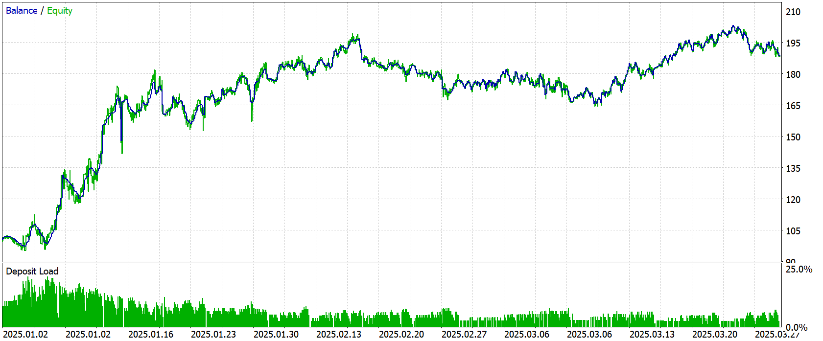
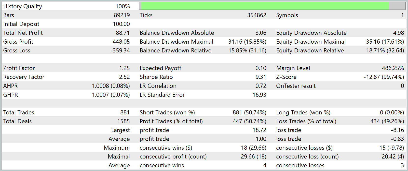
During the testing period, the model executed 881 trades, of which 447 were profitable, corresponding to a success rate of 50.74%. This indicates a neutral balance between profitable and losing trades. The profit factor (Profit Factor) is 1.25.

Overall, the strategy has delivered positive results with a moderate level of risk and steady equity growth during the first half of the testing period. However, after mid-February, profitability declines, and there is a clear sideways/range-bound movement with declining equity.

Thus, the strategy is viable and shows positive performance over the test interval; however, several parameters need improvement.

Conclusion

As a result of our work, we have fully integrated the Mantis framework into a customized algorithmic trading model capable of extracting informative features from high-frequency time series and converting them into meaningful decisions in real time.

Special attention was given to the self-supervised contrastive learning phase of the Encoder, implemented in the StudyContrast.mq5 EA. We moved away from a static dataset by implementing dynamic data loading from the terminal and enriching it with live examples from the past five years for the EURUSD M1 instrument. Positive and negative pairs, generated through soft augmentation and controlled noise, enabled the model, in practice, to learn to see through market noise.

Final testing of the model over the January–March 2025 period demonstrated the profitability of the implemented solutions. The strategy is viable and shows positive performance over the test interval; however, several parameters need improvement.

References

• Mantis: Lightweight Calibrated Foundation Model for User-Friendly Time Series Classification
• Other articles in this series

Programs used in the article

#	Name	Type	Description
1	Research.mq5	EA	EA for collecting examples
2	ResearchRealORL.mq5	EA	EA for collecting examples using the Real-ORL method
3	StudyContrast.mq5	EA	EA for contrastive training of the Encoder
4	Study.mq5	EA	EA for offline model training
5	StudyOnline.mq5	EA	EA for online model training
6	Test.mq5	EA	Model testing EA
7	Trajectory.mqh	Class Library	Structure for describing the system state and model architectures
8	NeuroNet.mqh	Class Library	Class library for building a neural network
9	NeuroNet.cl	Library	OpenCL program code library