From Basic to Intermediate: Queues, Lists, and Trees (V)

Introduction

In the previous article From Basic to Intermediate: Queues, Lists, and Trees (IV), we implemented a singly or doubly linked list. Although we have implemented a linked list, we can improve various aspects of this code model and make what was explained much easier to use. Thanks to these changes, the linked list now looks much more natural, and the code is easier to read and understand—at least, that is what I think.

To improve the code, we need to use some MQL5 resources that I have not mentioned yet. Since I do not want to make a topic that is already fairly confusing for many people even more complicated, I will show you later how to apply these changes to a linked list.

Now let's focus on our main topic: understanding the characteristics and differences between queues, lists, and trees. Since we are already approaching the last topic we will cover here, I can analyze some interesting aspects of these data structures. To that end, we will focus on the main topic of this short series of articles.

Queues, Lists, and Trees (V)

So, we have reached the fifth article, which focuses on queues, lists, and trees. Before we move on to the main issue of today's article, let's briefly review what we have already covered.

First, we learned what queues are, how they can be implemented, and what advantages they offer for organizing certain types of data or even events in general. However, queues have one significant drawback: we cannot arbitrarily insert new elements or remove existing ones. In other words, if you want to remove an element from the middle of the queue, you will not be able to do so—at least not quickly and efficiently. Adding new elements to the middle of the queue will not be very fast either.

That is why another type of data structure was created: the linked list. A linked list can be of two types: a singly linked list or a doubly linked list. Pointers link elements—which is not the case with queues—and allow elements to be added or removed with high efficiency at any position in the list. It is worth remembering that, in many cases, a list functions as an enhanced queue and performs the same functions, although it requires slightly more memory than a queue with the same number of elements.

So, if a list solves the problems with queues and can even replace them in many situations, why do we need trees? And what role do they play in all of this? Well, dear reader, trees are the natural evolution of lists, and they serve an even more important purpose. "Okay, but I still don't get it. Could you explain that in more detail before we start discussing the code?" Of course I can. I think that understanding the purpose of trees before looking at the code will help you understand the code itself. To understand trees, you need to understand the problem with lists. Yes, and although they solve the problem with queues, lists themselves have their own problems. For this reason, another data structure was created that makes it possible to search for elements more efficiently. Not clear yet? How is that possible?

To understand this, imagine lists containing thousands, perhaps even billions, of elements—a number that might seem unimaginable to most people. However, even lists containing several thousand elements can cause problems when searching. The main problem is the time the search takes.

Consider the following: you decide to put an entire dictionary into a list to create a text-checking system, and you implement a system that searches starting with A and proceeds word by word all the way to the last word beginning with Z. At first glance, this method seems practical and viable. However, in practice, this is not the case, because searching for specific words can take quite a long time. Now, if you modify the implementation so that the search sometimes starts with A and sometimes with Z, then in the worst-case scenario, you will have to go through half the list before the word you are looking for is found. This improvement may seem very positive, and perhaps it is. However, we can improve it even further. If, instead of sometimes starting at the beginning and sometimes at the end, we could start in the middle of the list, the number of elements we would have to check during a search would be significantly smaller, even in a fairly large list. In that case, we would have to go through about a quarter of the list, since, depending on the position chosen as the center, there may be more or fewer elements on one side or the other.

I think you are now starting to understand what gave rise to trees. Theoretically, a list does not form a tree. In practice, however, a list with a small number of elements arranged in a certain way can in fact be seen as a tree, albeit an unbalanced one.

Now, dear reader, you need to understand a very important point. There are various types of trees, and each one serves a specific purpose. Depending on the purpose, a tree may differ significantly from the one we will examine here, since explaining all types and their possible implementations would require a large number of articles. Since my intention here is simply to introduce this data structure for future use, each reader will have to study the other types of trees on their own and determine when it is appropriate to use each one. Here, I will present and explain a general tree model. However, as I mentioned earlier, I recommend that you explore this topic and look into other tree implementation models. Depending on the task you need to tackle, you will probably find a more suitable model.

All right, let's start with the following theoretical representation of a very simple tree.

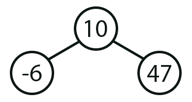
Figure 01

"How strange. I think I've seen something similar to Figure 01 before." Indeed, dear reader, Figure 01, which theoretically represents a tree, can also be found in other programming-related topics. You have probably come across a similar diagram if you studied the data structures used in artificial intelligence. However, in this field, another, even more advanced data structure than trees is typically used: GRAPHS. For now, we will not be discussing GRAPHS, since that would require delving into an approach and methodology that, in my opinion, many people are not yet ready to understand.

Nevertheless, we can implement artificial intelligence using trees without delving into graphs. To be honest, it is entirely possible to do that. But since we have only just begun discussing this topic, let's take it one step at a time.

All right, you need to understand an important classification issue that is directly related to Figure 01. The problem is this: when looking at Figure 01, and after you have understood what a queue is and what a list is, you might question my claim that the structure shown in Figure 01 is a tree. And you would not be wrong; on the contrary, you would demonstrate that you have a thorough understanding of the characteristics of queues and lists, since the structure shown in that same Figure 01 can be implemented using data structures that are not necessarily trees. All right, then what would you say about the image below?

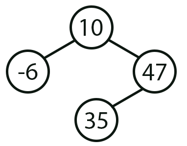
Figure 02

Now we have a tree. Actually, not yet, dear reader. Just like the structure shown in Figure 01, the structure in Figure 02 can also be implemented using a non-tree data structure. Now take a look: these two images illustrate a problem that many beginners overlook—they often look for much more complicated solutions to relatively simple problems. We need to implement a tree when, while modeling data or the elements being analyzed, we obtain a structure similar to the one shown in Figure 03 below:

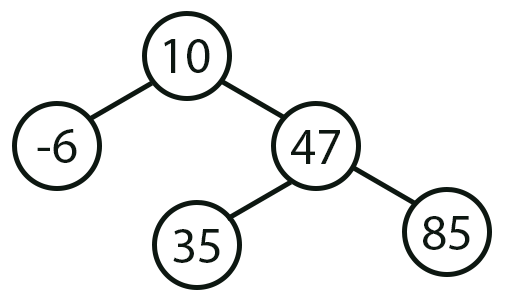
Figure 03

Now pay extra attention, because this will help you understand what we are going to implement. Notice that in the first two figures, there was only a single line connecting the elements. Although there are trees constructed in this way, they can also be implemented using simpler data structures, such as a queue or even a list. However, the structure shown in Figure 03 is different: at a certain point, a branch appears that allows us to take a different path without moving the other elements from their respective positions. It is precisely this branching that leads to the formation of a tree. Usually, in simple implementations like the one we will look at here, there are only two possible paths. However, in some systems—for example, when using artificial intelligence—there may be multiple paths originating from a single element. But we are still working with trees.

To make this easier to understand and explain, we'll use a few terms. If a point contains any element, we will refer to that point as a node. We will refer to the path we take to reach another element as a branch. There is also another term for the initial element, or initial node, of a tree. This element has a special name: the root.

Before we look at the code, let's analyze one more aspect of the structure. The terms “node” and “branch” are simple and practical. However, this does not apply to the root. Designating a particular node as the root completely changes the tree's characteristics. Changing the root node often significantly speeds up searches in the tree. In other cases, we are not concerned with search speed, but rather with the classification of elements. This explains the existence of artificial intelligence implementations that use trees. But again, let's take it step by step. It is still too early to talk about that.

Since our purpose here is educational and Figure 03 already shows our first tree diagram, we can implement the structure represented by this figure in our code. Keep in mind that here I'll show you how to do this in the most general way possible.

To begin with—at least at first—a tree is not all that different from a doubly linked list. You will understand this better soon. So we can start with the code we saw in the previous article, which is reproduced below.

001. //+------------------------------------------------------------------+
002. #property copyright "Daniel Jose"
003. //+------------------------------------------------------------------+
004. template <typename T> class stList
005. {
006.     private:
007. //+----------------+
008.         T info;
009.         stList <T>  *prev,
010.                     *start;
011.         uint        counter;
012. //+----------------+
013.     public:
014. //+----------------+
015.         stList(void)
016.             :prev(NULL),
017.             start(NULL),
018.             counter(0)
019.         {}
020. //+----------------+
021.         void Store(T arg, const uint index = 0xFFFFFFFF)
022.         {
023.             stList <T> *loc,
024.                         *ptr1 = start,
025.                         *ptr2 = NULL;
026. 
027.             for (uint c = 0; (ptr1 != NULL) && (c < index); ptr2 = ptr1, ptr1 = (*ptr1).start, c++);
028. 
029.             loc = new stList <T>;
030.             (*loc).info = arg;
031.             (*loc).start = (ptr2 != NULL ? (*ptr2).start : ptr1);
032.             (*loc).prev = (ptr1 != NULL ? (*ptr1).prev : ptr2);
033.             if (ptr2 != NULL) (*ptr2).start = loc; else start = loc;
034.             if (ptr1 != NULL) (*ptr1).prev = loc; else prev = loc;
035. 
036.             counter++;
037.         }
038. //+----------------+
039.         bool Restore(T &arg, const uint index = 0xFFFFFFFF)
040.         {
041.             if ((prev == NULL) || (start == NULL))
042.                 return false;
043. 
044.             stList <T>  *loc = (index < counter ? start : prev),
045.                         *ptr = NULL;
046. 
047.             for (uint c = 0; (loc != NULL) && (c < index) && (index < counter); ptr = loc, loc = (*loc).start, c++);
048.             if (loc == NULL) return false;
049. 
050.             if (index == 0)
051.             {
052.                 start = (*loc).start;
053.                 if (start != NULL) (*start).prev = NULL;
054.             } else if (index >= (counter - 1))
055.             {
056.                 prev = (*loc).prev;
057.                 if (prev != NULL) (*prev).start = NULL;
058.             }
059.             else
060.             {
061.                 (*ptr).start = (*loc).start;
062.                 (*loc).start.prev = ptr;
063.             }
064.             arg = (*loc).info;
065.             delete loc;
066.             counter--;
067. 
068.             return true;
069.         }
070. //+----------------+
071.         bool Exclude(const uint index)
072.         {
073.             T tmp;
074. 
075.             return Restore(tmp, index);
076.         }
077. //+----------------+
078.         void Debug(void)
079.         {
080.             Print("===== DEBUG =====");
081.             for (stList <T> *loc = start; loc != NULL; loc = (*loc).start)
082.                 PrintFormat("0x%06X ->> 0x%06X <<- 0x%06X = [%d]", (*loc).start, loc, (*loc).prev, (*loc).info);
083.             Print("=================");
084.         }
085. //+----------------+
086. };
087. //+------------------------------------------------------------------+
088. void OnStart(void)
089. {
090.     stList <char> list;
091. 
092.     list.Store(10);
093.     list.Store(84);
094.     list.Store(-6);
095.     list.Store(47, 0);
096. 
097.     list.Debug();
098. 
099.     list.Exclude(3);
100.     list.Store(35, 2);
101. 
102.     list.Debug();
103. 
104.     for (char info; list.Restore(info, 0);)
105.         Print(info);
106. };
107. //+------------------------------------------------------------------+

Code 01

It is clear that Code 01 implements a doubly linked list. However, if we modify this same code slightly, we can implement the tree shown in Figure 03. It is not difficult for experienced programmers to make changes to it, but it is more challenging for beginners or those with little experience—which is probably the case for many of you. And please do not get discouraged when you read this, because I was once in the same situation you are in now. However, thanks to study and a considerable amount of practice, I developed a solid level of understanding.

Since converting Code 01, which implements a doubly linked list, into a tree requires an understanding of various concepts that have not yet been explained in this series, we will take a different approach. In this way, we will maintain the educational nature of the explanation.

So we will start with a very simple and functional implementation, even though it does not yet support all tree operations. This code is shown below:

01. //+------------------------------------------------------------------+
02. #property copyright "Daniel Jose"
03. //+------------------------------------------------------------------+
04. class stTree
05. {
06.     public:
07.         int     info;
08.         stTree  *left,
09.                 *right;
10. };
11. //+------------------------------------------------------------------+
12. stTree *store(stTree *root, stTree *r, int info)
13. {
14.     if (r == NULL)
15.     {
16.         r = new stTree;
17. 
18.         (*r).left = NULL;
19.         (*r).right = NULL;
20.         (*r).info = info;
21.         if (root == NULL) return r;
22.         if (info < (*root).info) (*root).left = r;
23.         else (*root).right = r;
24. 
25.         return r;
26.     }
27.     if (info < (*r).info) return store(r, (*r).left, info);
28.     return store(r, (*r).right, info);
29. }
30. //+------------------------------------------------------------------+
31. void inorder(stTree *root)
32. {
33.     if (root == NULL) return;
34. 
35.     inorder((*root).left);
36.     if (root != NULL) Print((*root).info);
37.     inorder((*root).right);
38. }
39. //+------------------------------------------------------------------+
40. void OnStart(void)
41. {
42.     stTree *root = NULL;
43. 
44.     root = store(root, root, 10);
45.     store(root, root, -6);
46.     store(root, root, 47);
47.     store(root, root, 35);
48.     store(root, root, 85);
49. 
50.     inorder(root);
51. }
52. //+------------------------------------------------------------------+

Code 02

Do not worry about Code 02. I understand that the way this works probably intimidates you a little. However, we are not doing anything fundamentally new here. Perhaps the code simply shows these elements in a slightly different way. All the parts that appear in Code 02 have already been explained in other articles in this series. After running the program in the MetaTrader 5 terminal, you will see the following:

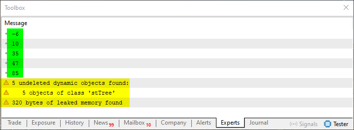
Figure 04

In Figure 04, I highlight two points. The text highlighted in yellow is a MetaTrader 5 warning indicating that the memory allocated by the statement on line 16 of Code 02 is not being returned to the system. However, for now, we can ignore these warnings, since they have no effect on the result obtained. The data highlighted in green are what really interests us, since they correspond to the result obtained by running the code that implements the tree shown in Figure 03.

"But wait a second. How is that possible? In Figure 03, we see a tree, but this area, highlighted in green in Figure 04, appears to me to be a list of values." And that is indeed the case, dear reader. However, there is a way to show that we are working with a tree here, not a list. We can demonstrate this by traversing the tree in different orders without much effort. But before we demonstrate that, let's quickly go over how Code 02 works. If you look closely, you will see that inside the OnStart procedure we use a function to build the tree structure and a procedure to traverse it and display its values.

But how does all this work? To begin with, note the structure declaration on line 04. Note that although we use the word “class” here, you should understand it as a structure. Here, we have two pointers: one for the right branch and the other for the left branch. We could have many more pointers like this, but here we will limit ourselves to the simplest and most basic option. After defining this structure, which is very similar to the one in Code 01, we can move on to implementing the tree-building function declared on line 12 of Code 02.

This function is recursive. In the article From Basic to Intermediate: Recursion, we discussed what recursion is. The recursive calls are exactly on lines 27 and 28. The if-statement block on line 14 allocates memory and inserts new nodes into the tree. Essentially, this block of code works very similarly to the block between lines 29 and 34 of Code 01. However, here in Code 02, the instructions between lines 14 and 26 create and insert a new node into the tree. But there is one thing to keep in mind. Unlike a linked list, where we specified the position at which an element was inserted, here we compare the value to be inserted with the values stored in the existing nodes of the tree. This allows us to construct a binary search tree.

"Hmm, I think I get it. That's why you said that when building a tree, we need to determine exactly what we want to achieve. That is why, when we traverse the tree, we see the data in the correct order."

Well, something like that, dear reader. However, the tree's elements are not necessarily organized in the way you might expect. In fact, the traversal routine declared on line 31 returns the elements in ascending order during tree traversal. "But wait a second. How is that possible? Now I am completely confused. You just said that the function on line 12 orders the elements as the tree is being built. Indeed, if we look at the conditions, assignments, and recursive calls on lines 22, 23, 27, and 28, we can see that elements with smaller values will remain in the left branches, while elements with larger values will be directed to the right branch. I thought that would be enough to order the elements within the tree. But now you are saying that the traversal procedure returns elements in ascending order. To me, that makes absolutely no sense."

Do not worry, dear reader; you will understand everything soon enough. But first, note the following: the recursive procedure declared on line 31 will start at the root node and keep looking for the leftmost element until it can no longer find one. The recursive call on line 35 continues the search in the left subtree. When this call completes, we will display the value of the current node. Next, we will start a new search, but this time to the right, using a recursive call on line 37. When entering the right subtree, the procedure will again make the call on line 35, allowing it to check the new branch on the left.

Here, we will traverse the tree and examine its elements in a specific order. When constructing the tree, we place elements with smaller values to the left of elements with larger values and establish an ordering relation that becomes apparent only when the tree is traversed in a specific way.

However, if we change the way we traverse the tree, we may get a completely different result. To test this, let's take a look at the following code.

01. //+------------------------------------------------------------------+
02. #property copyright "Daniel Jose"
03. //+------------------------------------------------------------------+
04. class stTree
05. {
06.     public:
07.         int     info;
08.         stTree  *left,
09.                 *right;
10. };
11. //+------------------------------------------------------------------+
12. stTree *store(stTree *root, stTree *r, int info)
13. {
14.     if (r == NULL)
15.     {
16.         r = new stTree;
17. 
18.         (*r).left = NULL;
19.         (*r).right = NULL;
20.         (*r).info = info;
21.         if (root == NULL) return r;
22.         if (info < (*root).info) (*root).left = r;
23.         else (*root).right = r;
24. 
25.         return r;
26.     }
27.     if (info < (*r).info) return store(r, (*r).left, info);
28.     return store(r, (*r).right, info);
29. }
30. //+------------------------------------------------------------------+
31. string inorder(stTree *root)
32. {
33.     static string sz0 = "In Order: ";
34. 
35.     if (root == NULL) return sz0;
36. 
37.     inorder((*root).left);
38.     sz0 += (root != NULL ? StringFormat("%d  ", (*root).info) : "");
39.     inorder((*root).right);
40. 
41.     return sz0;
42. }
43. //+------------------------------------------------------------------+
44. string preorder(stTree *root)
45. {
46.     static string sz0 = "Pre Order: ";
47. 
48.     if (root == NULL) return sz0;
49. 
50.     sz0 += (root != NULL ? StringFormat("%d  ", (*root).info) : "");
51.     preorder((*root).left);
52.     preorder((*root).right);
53. 
54.     return sz0;
55. }
56. //+------------------------------------------------------------------+
57. string postorder(stTree *root)
58. {
59.     static string sz0 = "Post Order: ";
60. 
61.     if (root == NULL) return sz0;
62. 
63.     postorder((*root).left);
64.     postorder((*root).right);
65.     sz0 += (root != NULL ? StringFormat("%d  ", (*root).info) : "");
66. 
67.     return sz0;
68. }
69. //+------------------------------------------------------------------+
70. void OnStart(void)
71. {
72.     stTree *root = NULL;
73. 
74.     root = store(root, root, 10);
75.     store(root, root, -6);
76.     store(root, root, 47);
77.     store(root, root, 35);
78.     store(root, root, 85);
79. 
80.     Print(inorder(root));
81.     Print(preorder(root));
82.     Print(postorder(root));
83. }
84. //+------------------------------------------------------------------+

Code 03

Now, pay close attention, dear reader. Note that Code 03 has not changed if compared to Code 02. However, we have added two new functions for traversing the tree in different ways and displaying its values. These functions are declared on lines 44 and 57. Since the output will now be longer, I have tweaked the code a bit so that it returns a string, making it easier to read.

In this case, trace through the OnStart procedure. Virtually everything has remained the same as in Code 02. However, when we run Code 03, we get the result shown in the following figure:

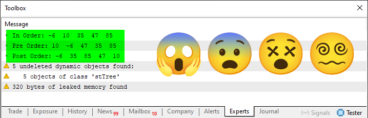
Figure 05

Once again, the part we are interested in is highlighted in green in Figure 05. Note that even if we build the tree in the same way, the result will depend on both the type of traversal and the order in which we insert the values. "But why is that? I didn't understand what you just said." Do not worry. Please be patient; we will get to that in a moment. First, let's analyze the information in Figure 05. Please note that it contains a line of values in ascending order, generated by the call in the statement on line 80 of Code 03. We also have preorder values and postorder values. Each of these lines corresponds to a different tree traversal. To explain why the insertion order causes these traversals to produce different sequences, we will change one small detail in Code 03. This is shown in the following snippet:

                   .
                   .
                   .
69. //+------------------------------------------------------------------+
70. void OnStart(void)
71. {
72.     stTree *root = NULL;
73. 
74.     root = store(root, root, 10);
75.     store(root, root, -6);
76.     store(root, root, 85);
77.     store(root, root, 35);
78.     store(root, root, 47);
79. 
80.     Print(inorder(root));
81.     Print(preorder(root));
82.     Print(postorder(root));
83. }
84. //+------------------------------------------------------------------+

Snippet 01

Now take a look at the result shown below:

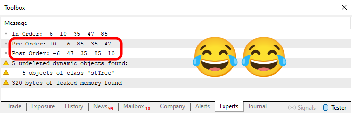
Figure 06

This is rather curious. Please note that the change in the code is very minor—practically imperceptible—but the result may differ significantly from what you expect. I struggled a lot when I was just starting out as a programmer and ran into situations like that. Many people are not aware of this or do not understand it. But if you compare the elements generated by the traversal shown on the "Pre Order" line, you will notice that they appear in exactly the same order in which we added them. It is crazy, isn't it? That is why I mentioned at the beginning of this article that trees should be studied very calmly and carefully.

Do not think you have already mastered the topic just because you know how to write a particular piece of code. This type of data structure is indeed very interesting and has many applications in various fields and domains related to data analysis.

Concluding Thoughts

In this article, we implemented the first components of a tree structure. Since I know this structure can seem extremely complicated when you are just starting to learn it, I won't go any deeper into it in this article. We will go through this step by step, although ultimately we will implement and demonstrate only a basic and general tree structure.

However, I want to pique your curiosity, dear reader, so that you understand that there are simple data structures that allow you to perform operations efficiently and obtain specific results. To do this, you need to have a very good understanding of how a tree is structured. This will give you an understanding of the data structure for artificial intelligence that we will soon be implementing: it will be both fascinating and simple, and the way it works will prove truly amazing.

Therefore, please study this article and the previous ones carefully to fully understand the structures and procedures described here. In the next article, we will implement more components of this generalized tree structure.

MQ5	Description
Code 01	A Simple Tree
Code 02	A Simple Tree
Code 03	A Simple Tree