MQL5 Wizard Techniques you should know (Part 87): Volatility-Scaled Money Management with Monotonic Queue in MQL5

Introduction

Algorithmic traders and MQL5 Expert Advisor developers often face a specific, reproducible failure mode: strategies that work in backtests collapse in live or low‑latency environments when market range expands. The root cause is usually static position sizing (fixed lots or fixed‑percent rules) combined with delayed volatility estimates: sliding‑window routines (brute‑force scans, heaps, or repetitive CopyHigh/CopyLow calls) introduce measurable latency on VPS instances, especially at low timeframes or when trading multiple symbols. The consequence is clear and quantifiable — oversized risk during news spikes or thin liquidity, larger single‑trade losses, and deeper equity drawdowns.

This article proposes a practical, deployable remedy: a zero-lag money-management pipeline that (1) computes Donchian-style range extremes in O(N) using a Monotonic Queue (deque) to eliminate sliding-window latency, and (2) applies a lightweight Radial Basis Function (RBF) gatekeeper to nonlinearly validate signal quality before finalizing lots. The deliverable is a ready‑to‑integrate MQL5 module (CMoneyMonotonicQueueRBF::Optimize) with tunable inputs (window size, m base volatility, use rbf) that (a) produces an instantaneous current volatility, (b) computes scale factor = base volatility / current_volatility, (c) normalizes lots to broker step/min/max, and (d) — optionally — multiplies by an RBF output in [0,1]. The approach targets EA developers who require preventive, real‑time risk scaling and a reproducible test protocol for Strategy Tester comparisons.

Problem

Position sizing should look beyond fixed lots and fixed-percent options. Further to this, depending on the compute resources available on the hosting VPS, introducing real-time volatility measurement to this decision-making can be hampered by compute latency. Traditional sliding-window calculations on volatility can lead to this latency, especially in high-frequency/low-timeframe trading environments. Standard Donchian channel implementations often use brute-force array sorting with O(N) complexity meaning more execution delays as the lookback window increases. For many trading systems, even a few milliseconds of delay can affect order placement speed and the ability to minimize slippage-induced losses.

Compounding this further is the retrospective approach to managing risk. Most risk management methods are legacy in that they evaluate/analyze historical trade outcomes as opposed to focusing on the now, real-time market microstructure. Algorithms that depend on reducing volume used from consecutive loss counts, tend to lag, since they do not scale risk against expanding volatility vectors. The triggering of the ‘Decrease Factor’ after a failed sequence of trades often occurs after the account has absorbed most of the impact from the market shift.

To address these failures, this article proposes a shift towards ‘zero-lag’ money management. This approach is necessary because of the need for efficient risk adjustment that anticipates volatility rather than reacting to realized losses. The importance of this thesis lies in the introduction of a dual-layered defense mechanism. Our approach uses a high-efficiency monotonic queue for real-time volatility tracking and a radial basis function network for non-linear risk validation. This article argues that by bringing together advanced computer science data structures and machine learning, traders can achieve improvements in capital preservation, that is optimized for the compute demands of today's financial markets.

Algorithmic Optimization – The Monotonic Queue Mathematics

Real-time volatility tracking can introduce significant compute overhead, which is often a main constraint for traders who want to embark on high-frequency/low-timeframe trading. To derive the metrics for measuring volatility from indicators such as the Donchian Channel, a trade system needs to identify maximum and minimum price points within a rolling window of length K. Traditional brute-force methods usually necessitate a complete scan of the window, sized K, resulting in a time complexity of O(N.K). Even if the optimized methods of binary search trees or heaps are used, the complexity still remains O(N * logK). These methods can be enough for low-frequency applications however, if one’s system processes more than one symbol, on a very low timeframe then they can introduce non-negligible latency.

The Monotonic Queue does give us a mathematically superior solution by enabling sliding window extremes discovery with a total time complexity of O(N). This efficiency is possible by maintaining a double-ended queue (deque) where elements are kept in a strict monotonic order. By ensuring that the elements are sorted, either in decreasing maximums or ascending minimums, for any given lookback window, this allows O(1) access time.

The monotonic queue's efficiency is explained through amortized analysis. Every element within the price series is pushed into the queue exactly once and popped from the queue no more than once. Although the push operation uses nested loops to preserve monotonicity, the total number of operations across N elements is bounded by 2N. This reduces the complexity from multiplying with the history window size of K to a purely linear relationship that's set by the total number of data points N.

Comparison Table

Algorithm	Time Complexity (per update)	Total Complexity (N elements)	Latency Sensitivity
Brute-Force	O(K)	O(N . K)	High
Max Heap/BST	O(log K)	O(N log K)	Moderate
Monotonic Queue	O(1) (Amortized)	O(N)	Minimal

By leveraging this data structure, the money management custom class can update its volatility parameters almost immediately once a new quote is received. This allows us to have the risk scaling logic operating on the most current market microstructure with minimal lag.

The implementation of the ‘CMonotonicQueueMax’ Class within the custom mm class serves as our backbone within this custom class. High-speed is a key factor but also is memory efficiency. We construct this class as follows:

    CMonotonicQueueMax(int window) : m_head(0), m_tail(0), m_window(window)
     {
      ArrayResize(m_deque_values, window);
      ArrayResize(m_deque_indices, window);
     }

The constructor does a pre-allocation of memory for the ‘m_deque_values’ as well as ‘m_deque_indices’ arrays. Since we resize the arrays to the exact window size at initialization, the system avoids performance penalties often linked with dynamic memory reallocation midway through trading sessions.

The push method is where the O(1) amortized logic is set in place thanks to two important validation loops. This is shown in the code below:

   void              Push(int index, double value)
     {
      // Remove elements not within the temporal window
      while(m_head < m_tail && m_deque_indices[m_head] <= index - m_window)
         m_head++;
      // Remove sub-optimal elements to maintain strict monotonic decreasing order
      while(m_head < m_tail && m_deque_values[m_tail - 1] <= value)
         m_tail--;
      // Append current element
      m_deque_values[m_tail] = value;
      m_deque_indices[m_tail] = index;
      m_tail++;
     }

The first loop sees to it that the data remaining in the queue is temporally relevant. If the index of the element at the head of the queue is less than or equal to the current index less the window size, then that data point has expired, and the head point gets incremented. The second while loop maintains the monotonic decreasing order. Prior to a new value being added, it is compared against the values at the tail. If the existing tail value is less than or equal to the value that is incoming, it gets discarded, or the tail pointer gets decremented. The math logic behind this is a smaller, older value can never be the max if a larger newer value is in the same window.

In wrapping up, the new value and its corresponding index are recorded at the current tail position. The tail position then gets incremented. Because the Push function maintains a strictly decreasing order, the largest value is always at m head, enabling O(1) retrieval of highs for the volatility calculation. Notably, we do not have a CMonotonicQueueMin class in our code as a deliberate shortcut since fundamentally the math property below holds and is exploited within the code:

min(x) = -max(-x)

MQL5 Implementation of the Custom Money Management Class

The shift from a theoretical O(N) data structure to a working one in the MQL5 Custom Money Management module is done with the ‘Optimize()’ function of this class. At this point we examine how real-time volatility scaling is used to adapt and adjust the position sizing. The Optimize function is as follows:

//+------------------------------------------------------------------+
//| Optimizing lot size via Monotonic Queue and RBF Gatekeeper       |
//+------------------------------------------------------------------+
double CMoneyMonotonicQueueRBF::Optimize(double lots)
  {
   double lot = lots;
   double current_volatility = 0.0;
   if(m_window_size > 0)
     {
      double high[], low[];
      ArraySetAsSeries(high, true);
      ArraySetAsSeries(low, true);
      // 1. $O(N)$ Monotonic Queue Volatility Extraction
      if(CopyHigh(m_symbol.Name(), PERIOD_CURRENT, 0, m_window_size, high) == m_window_size &&
         CopyLow(m_symbol.Name(), PERIOD_CURRENT, 0, m_window_size, low) == m_window_size)
        {
         CMonotonicQueueMax mq_high(m_window_size);
         CMonotonicQueueMax mq_low_inverted(m_window_size);
         for(int i = m_window_size - 1; i >= 0; i--)
           {
            mq_high.Push(m_window_size - 1 - i, high[i]);
            mq_low_inverted.Push(m_window_size - 1 - i, -low[i]);
           }
         double max_high = mq_high.Max();
         double min_low = -mq_low_inverted.Max();
         current_volatility = max_high - min_low;
         // Volatility scaling logic
         if(current_volatility > m_base_volatility && current_volatility > 0)
           {
            double scale_factor = m_base_volatility / current_volatility;
            lot = NormalizeDouble(lot * scale_factor, 2);
           }
        }
      // 2. Non-Linear RBF Risk Validation
      if(m_use_rbf)
        {
         if(m_handle_rsi != INVALID_HANDLE)
           {
            double rsi_buffer[1];
            if(CopyBuffer(m_handle_rsi, 0, 0, 1, rsi_buffer) == 1)
              {
               // Construct State Vector: Normalize inputs for the Gaussian kernel
               double state_vector[2];
               state_vector[0] = MathMin(current_volatility / (m_base_volatility * 5.0), 1.0); // Normalized Volatility
               state_vector[1] = rsi_buffer[0] / 100.0;                                        // Normalized RSI
               // Gatekeeper Output: Multiply current lot by the probability coefficient
               double rbf_coefficient = m_rbf.Calculate(state_vector);
               lot = NormalizeDouble(lot * rbf_coefficient, 2);
              }
           }
        }
     }
//--- Broker compliance limits
   double stepvol = m_symbol.LotsStep();
   lot = stepvol * NormalizeDouble(lot / stepvol, 0);
   double minvol = m_symbol.LotsMin();
   if(lot < minvol)
      lot = minvol;
   double maxvol = m_symbol.LotsMax();
   if(lot > maxvol)
      lot = maxvol;
   return(lot);
  }

The implementation starts with declaring dynamic buffers that hold the price extremes. We ensure the arrays are series which means the arrays follow the indexing convention of where the most recent candle at index 0 aligns with the current market state/price(s). We check that CopyHigh and CopyLow return at least m window size values; otherwise, Optimize exits early. This effectively is a safety gate to prevent array-out-of-range exceptions, down stream.

Within the ‘Optimize’ method, two instances of the `CMonotonicQueueMax’ class are declared. Our for loop goes through the fetched price data to populate these structs. The inclusion of ‘mq_low_inverted’ has already been talked about above with the shared formula. By pushing the negative value of the low prices (‘-low[i]’), the standard ‘Max-Queue’ logic is changed to find the period minimum without having us code a parallel ‘Min-Queue’ or CMonotonicQueueMin class. This reduces our code’s complexity without compromising on the ‘math rigor’.

This leads us to the volatility extraction and scaling logic. This portion comprises our main “inverse-scaling” logic. Our method compares the real-time range against the Expert Advisor, tuned input parameter of m_base_volatility. Once a market expansion is detected, a scale factor is generated. By performing a product of the initial lot size with this factor the Expert Advisor ensures monetary risk stays relatively constant in spite of price gaps increasing. As an example, if volatility is to double relative to the baseline, the lot size would be halved.

The calculations at the end of this Optimize function ensure that our derived lot size is execution ready. We normalize the volume to the symbol’s ‘Lot Step’ and enforce hard limits that are based on the minimum lot size as well as the max lot size. This helps avert illegal trade volumes that would be rejected at the broker’s server.

Non-Linear Risk Validation - The RBF Network

Whereas the monotonic queue gives us a compute optimal framework for tracking physical market expansion, a validator of this monotonic queue lot scaling should be a model capable of interpreting non-linear structures. We elect to use a Radial Basis Function (RBF) Network, as an intelligent filter, categorizing the outputs of the ‘volatility-engine’ against trend following and oscillating indicators.

An RBF is a specialized form of artificial neural network that engages radial basis functions as activation functions. While Multi-Layer Perceptrons use global approximation, the RBF network uses local approximation making it uniquely suited for financial time-series data that usually features regime shifts. The RBF network structure usually is made up of three layers: 

• The input layer: We provide a vector of real-valued inputs (double data type) which include the current monotonic queue bandwidth. As an alternative, indicator readings from the RSI, or even Envelope Deviations can also be supplemented
• The hidden layer: This is a collection of neurons where each neuron performs a Gaussian Radial Basis function.
• The output layer: This serves as our linear combination of the hidden layer outputs. It provides the final risk scaling coefficient.

Mathematically, the Gaussian kernel, which defines the hidden layer’s ‘response’ is represented as follows:

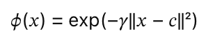
Where:

• X is the input vector
• C is the center of the specific neuron
• Gamma is the parameter controlling the width of the bell-curve

The RBF network computes the Euclidean distance between the live market state as well as its learned ‘profit-centers’. This ensures that volume is only allocated when the current market geometry matches a known statistical edge.

Our choice of using an RBF instead of alternative deep learning architectures is motivated by two science based factors:

• Convergence speed: The RBF hidden layer parameters can be set through unsupervised learning (i.e. clustering). This allows for significantly faster training cycles within the MQL5 environment, versus standard backpropagation.
• Rejection of anomalous data: Because of the local nature of the Gaussian function, if the market state gets into a new zone or unchartered waters such as a ‘black-swan’ volatility, the activations of the neurons would decrease towards zero.

Implementing the RBF, in our custom money management class, has us set it up as a ‘gate-keeper’. We have it situated between the initial lot calculation and the last execution. This process follows the following deterministic sequence:

• The monotonic queue sets the lot size while using the afore mentioned inverse volatility scaling
• The RBF Network then receives the state vector which from our code receives volatility and a normalized reading of the RSI.
• The network outputs a value between 0.0 and 1.0.
• The final lot size prior to processing the RBF, then gets multiplied by this RBF coefficient.

If the market environment is high-volatility but the RSI indicates an over extended condition which the RBF network marks as a low-probability entry, the RBF output factor would then truncate the lot size even further. What this does is ensure that the Expert Advisor is not merely reacting to the ‘size’ of the market volatility but rather it is also evaluating the ‘signal-quality’ via probability distribution, thus giving us a multi-dimension approach to capital preservation.

Empirical Backtests

In order to substantiate our theoretical arguments for the monotonic queue framework a comparative performance analysis can be resourceful. We use the MetaTrader 5 Strategy Tester. Our objective here is to isolate the impact of the volatility-scaling algorithm by keeping an identical signal logic of the RSI and Envelopes across a control custom money management class and the experiment mm class. The statistical divergence between these two reports does serve as some evidence of system’s ability to mitigate risk without altering the underlying trade frequency.

The control report was based on an Expert Advisor that uses the built-in or IDE provided Size-Optimized money management. This built-in class reduces lots after an Expert Advisor sustains losses. It lacks real-time volatility sensitivity. The report, from 2023.03.01 to 2026.04.15, post optimization, on the symbol GBP/JPY is given below:

The system executed 16 trades resulting in a net profit of -1,730. This negative outcome is reflected in a profit factor of just 0.58, meaning the strategy’s gross losses significantly outweighed the gross gains. The maximum equity drawdown reached a critical level that was over 30%. A granular review of the trade list shows that the largest loss trade reached -1,193. This can be argued to mean that because we had no volatility inverse scaling, the EA maintained an outsized volume in a period of market expansion. This resulted in this single adverse movement inflicting disproportionate damage to the account equity. We also ran tests with the monotonic queue algorithm that was backed with the RBF Network filter. It presented us with the following report: 

The test report above outlines a performance of the same entry signal as the report presented above before it. We use a different money management ‘CMoneyMonotonicQueueRBF’ class. Perhaps the standout feature from this report is the stability of the trade count. Exactly 16 trades were executed suggesting volume allocation had a fair influence on the reported trade results. The EA successfully pivoted from a loss-making trajectory to profit, generating a net profit of 463.18. The profit factor also improved to 1.44 with a positive expected payoff of 28.95. The maximum Equity Drawdown compressed to 12.19%.

Our forward-walk runs for both the control report and this test report are from July 2025 to the test period end of 2026.04.15. The impact of the monotonic queue’s O(N) sliding window is very evident in the trade distribution. The largest loss trade was mitigated to -677.48 versus -1,193 that we had above. Therefore, it can be argued that by shrinking the lot size as the Donchian bandwidth expanded. This MM class effectively caps the monetary impact of unsuccessful entries particularly in high-volatility regimes.

The data from these two reports presents a clear correlation between algorithmic efficiency and capital preservation. The control group’s failure was not an issue of bad signals per se given the profit generated from the monotonic queue class with similar 16 entries. Differences in equity drawdown of 31% and 12% also mean that the monotonic queue fulfilled an important design requirement - it maintained a constant currency-at-risk. The inverse dynamic between market range and position size, calculated instantly via O(1) lookups.

Takeaways

The goal of this money management exploration was to bring together high efficiency of compute structures with adaptive risk-scaling logic, addressing inherent fragilities of non-adaptive money management. By introducing the ‘CMonotonicQueueRBF’ class, we have put in place a framework that systematically resolves the vulnerabilities spotted at the outset of our analysis. The integration of O(N) data structures and non-linear filtering represents a necessary evolution in the pursuit of capital preservation within non-stationary financial environments.

The central problem addressed here was the critical vulnerability of trading systems employing static volume in market expansion situations. This we resolve via the inverse scaling factor equation of:

scale_factor = m_base_volatility / current_volatility

As empirically demonstrated in the change from the control to the test EA, our Mathematical Scalar sees to it that as price ranges expand, position sizing contracts. This gives us a slightly more consistent currency-at-risk profile, that prevents disproportionate equity depletion typically observed in high impact market events.

The secondary problem we tackled was the unsustainable latency that is common in legacy sliding-window calculations. Through the application of the Monotonic Queue, we have reduced the complexity of volatility tracking from O(N.K) to O(N). By using the ‘Push’ method’s dual loop validation to maintain a strictly decreasing order, our system actually gets O(1) access to the period extremes. This eliminates the compute lag associated with brute-force array sorting ensuring that risk parameters get refreshed in sync with every new price bar.

Finally, the problem of depending on historical loss counters from trade history was overcome by shifting to real-time market microstructure. Instead of waiting for a sequence of realized losses to trigger volume reduction, our custom class uses Donchian Channel bandwidth tracking to anticipate risk. The Strategy Tester reports provide partial support for the pre-emptive method: 16 trades with a 12.19% drawdown versus 31% in the control report.

Conclusion

What this framework provides in practical terms is a reproducible, low‑latency money‑management blueprint and an MQL5 implementation ready for integration and testing. Key outcomes:

• Complexity reduction: sliding‑window max/min discovery is reduced from O(N K) or O(N log K) to amortized O(N) with O(1) per‑update access via a Monotonic Queue, enabling near‑instant volatility updates on each new quote.
• Deterministic scaling rule: position sizing is inversely adjusted by scale factor = base volatility / current_volatility, capping monetary exposure as market range expands.
• Signal quality gating: an optional RBF network maps normalized volatility and indicator state (eg, RSI) to a [0,1] coefficient that further moderates lot size when market geometry falls outside learned profit centers.
• Deliverables and integration points: the article supplies the CMoneyMonotonicQueueRBF class and the Optimize() routine (Calculate current volatility, apply scale factor, enforce lot step/min/max, apply RBF), plus guidance for embedding into MQL5 Wizard EAs.
• Testable metrics: compare net profit, profit factor, expected payoff, max equity drawdown, and largest single trade loss between control and MM‑enhanced runs using Strategy Tester.

Limitations and next steps: per‑call data copying (CopyHigh/CopyLow) and indicator buffer reads remain potential latency sources and should be profiled on target VPS hardware; RBF centers and gamma must be set or trained (clustering/unsupervised methods recommended) and validated out-of-sample. Nevertheless, by combining an O(N) volatility engine with a compact nonlinear gatekeeper, the framework gives EA developers a practical path toward anticipatory, zero-lag capital preservation in non-stationary markets.

name	description
wz_87_b	Wizard assembled Expert Advisor with Monotonic Queue Custom MM class
wz_87_ctrl	Wizard assembled Expert Advisor with built-in size-optimized MM
MoneyMonotonicRBF.mqh	Custom MM class based on Monotonic Queue
MoneySizeOptimized.mqh	Built-in IDE provided custom MM class

Attached code is meant to be assembled into an Expert Advisor by the MQL5 Wizard. There are guides here and here on how to do this for new readers.